Study design and participants
The UKB is a prospective cohort study with extensive genetic and phenotype data available for 502,505 individuals resident in the UK36. The full UKB protocol37 is available online. All statistical analyses were carried out using R v.4.2.2. and PLINK v.2.0.
Exposures
We considered all non-genetic variables available as of 24 July 2020 that were collected or derived (for example, air pollution and Townsend deprivation index) at baseline, had Supplementary Information and Supplementary Tables 9 and 10), 176 unique exposures remained that were available in the full cohort and were common to both women and men. All continuous exposure variables were centered and standardized before analysis, except for age at recruitment. All ordinal categorical variables were recoded to only test linear associations and other polynomial contrasts (for example, quadratic or cubic associations) were not assessed. All nominal categorical exposures were analyzed with the most common category set as the reference. All ‘mark all that apply’ questions were recoded as binary dummy variables. Detailed data dictionaries including all exposures used in imputation and XWAS steps are included in Supplementary Files 1 and 2.
Outcomes
Detailed information about the linkage procedure38 with national registries for mortality and cause of death information is available online. Mortality data were accessed from the UKB data portal on 4 May 2022, with a censoring date of 30 September 2021 or 31 October 2021 for participants recruited in England/Scotland or Wales, respectively (11–15 years of follow-up).
Procedures for calculating proteomic aging in the UKB were described previously19. Aging biomarkers (Supplementary Table 6) were measured using baseline nonfasting blood serum samples as previously described39. Data on leukocyte telomere length were only available in a slightly smaller sample (n = 472,506) than other biomarkers and were not imputed. Biomarkers were previously adjusted for technical variation by the UKB, with sample processing40 and quality control41 procedures described on the UKB website.
Data used to define prevalent and incident cases for chronic diseases and common disease risk factors are outlined in Supplementary Table 8. Incident chronic disease diagnoses were ascertained using International Classification of Diseases (ICD) diagnosis codes and corresponding dates of diagnosis taken from linked hospital inpatient records and death register data. ICD-9 and ICD-10 data were accessed from the UKB data portal on 30 May 2022, with a censoring date of 30 September 2021, 31 July 2021 or 28 February 2018 for participants recruited in England, Scotland or Wales, respectively (8–15 years of follow-up). Breast, ovarian and prostate cancer analyses were carried out as sex-specific analyses in female (breast and ovarian) or male (prostate) participants.
Missing data imputation
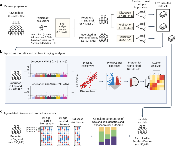
The average percentages of missing data across all final variables included in our UKB analysis datasets were 11% in women (range: 0–79%) and 10.9% in men (range: 0–77%). UKB participants recruited from England were randomly assigned to a discovery (n = 218,446) or replication set (n = 218,445) while maintaining the same proportion of mortality cases in each. We performed missing data imputation separately in the discovery, replication and Scottish/Welsh validation (n = 55,676) datasets using the R package missRanger42, which combines random forest imputation with predictive mean matching. We imputed five datasets, with a maximum of ten iterations for each imputation. We set the maximum number of trees for the random forest to 200, but left all other random forest hyperparameters at their default. The variables used as predictors in the imputation included all baseline, non-nested variables, the Nelson–Aalen estimate of cumulative mortality hazard and the all-cause mortality event indicator. All subsequent study analyses were run independently in each of the five imputed datasets, and results were pooled using Rubin’s rule43.
XWAS
XWAS of all-cause mortality were initially carried out separately in women and men, and then a final XWAS was calculated in the pooled dataset with both women and men to increase power. Exposures in the final pooled XWAS were limited to those applicable to both women and men, omitting sex-specific reproductive factors (only tested in the sex-specific XWAS). In each XWAS, we serially assessed associations of each individual exposure with all-cause mortality using Cox proportional hazards models with age as the timescale stratified by 5-year birth cohorts and sex (in the pooled analysis only), and adjusted for assessment center, years of education (7 years, 10 years, 13 years, 15 years, 19 years and 20 years) and ethnicity (white, Asian, Black, mixed or other). For each model, the baseline hazards were calculated separately in each of these strata, and resulting effect estimates are those that fit best across all strata. Since it has been shown that UKB participants are likely to misreport alcohol consumption as a function of higher disease burden44, self-reported overall health status was added as an additional XWAS covariate for the self-reported alcohol intake exposure only. P values in the discovery and replication analyses were corrected using the FDR (Benjamini–Hochberg method45) with a significance threshold of FDR P n = 436,891) to complete further sensitivity analyses.
Prevalent disease sensitivity analysis
We conducted a sensitivity analysis in the full sample of participants recruited in England (n = 436,891) where we individually tested every exposure replicated in the pooled mortality XWAS again in relation to mortality using the same XWAS formula and covariates, but now adding an interaction term between each exposure and an indicator of baseline disease or poor health (see definition below). We flagged and removed from further analysis any exposure that no longer had a significant direct effect in this model (P P
The baseline disease/poor health indicator was created for all participants, in which participants were coded as having disease or poor health at baseline if they (1) had a linked hospital inpatient ICD diagnosis for any of the chronic illnesses or common disease risk factors studied in our analysis (including hypertension, dyslipidemia and obesity) with a diagnosis date before or on their date of recruitment to the UKB; (2) were assigned a diagnosis code for any of the chronic diseases or common disease risk factors studied in our analysis during the baseline clinical interview (field IDs 20001 and 20002 in Supplementary Table 8); (3) self-reported a physician diagnosis of heart attack (field ID 6150), angina (field ID 6150), stroke (field ID 6150), high blood pressure (field ID 6150), bronchitis/emphysema (field ID 6152), diabetes (field ID 2443) or cancer (field ID 2453); (4) self-reported ≥1 cancer diagnoses (field ID 134); (5) self-reported taking insulin medication (field IDs 6153 and 6177), cholesterol lowering medication (field IDs 6153 and 6177) or blood pressure medication (field IDs 6153 and 6177); or (6) self-reported their overall health status as ‘poor’ (field ID 2178).
PheWAS of replicated exposures
For all exposures replicated in the XWAS and not removed during the above-described disease sensitivity analyses, a PheWAS was conducted. In each PheWAS, the exposure was used as the outcome variable (hereafter referred to as exposure outcomes) and was tested against the full set of baseline phenotypes available in the UKB (Supplementary File 62 provides the full list of phenotypes tested). Each PheWAS was conducted as a linear or logistic regression, depending on whether the exposure outcome was continuous or categorical, with covariates for age at recruitment and sex. All ordinal exposure outcomes were tested as continuous variables. Nominal categorical exposure outcomes were recoded into dummy variables for each response category versus the reference. All continuous phenotype exposures were scaled and centered to the mean before running the PheWAS. Summary statistics from all PheWAS are available in Supplementary Files 63–178.
Proteomic age clock analyses
We serially assessed associations between each exposure and proteomic age gap (the difference in years between plasma protein-predicted age and calendar age) using cross-sectional linear regression models with covariates for sex, age at recruitment, assessment center, years of education and ethnicity. In brief, we previously developed a proteomic age clock in a subset of UKB participants (n = 45,441) using a gradient boosting machine learning model that takes 204 proteins we identified and uses them to accurately predict chronological age (Pearson r = 0.94)19. In a validation study involving biobanks in China (n = 3,977) and Finland (n = 1,990), the proteomic age clock showed similar age prediction accuracy (Pearson r = 0.92 and r = 0.94, respectively) compared with its performance in the UKB. The proteomic age clock has been previously associated with the incidence of 18 major chronic diseases (including diseases of the heart, liver, kidney and lung, diabetes, neurodegeneration and cancer), as well as with multimorbidity and all-cause mortality risk.
Correlation and cluster analyses
Correlation between all variables was calculated in the full sample of participants recruited in England using the R package polycor46 to create a heterogeneous correlation matrix for each imputed dataset. Correlation coefficients were first calculated within each imputed dataset, transformed to a normally distributed z-score via Fisher’s z transformation, pooled via Rubin’s rule and then retransformed back to the original r-scale coefficient after pooling. We used hierarchical clustering via Euclidean distance to identify the cluster structure of exposures replicated in the pooled XWAS and not susceptible to reverse causation bias (plus education and ethnicity). We used within-cluster sum of squares (WSS) analyses to identify candidates for the optimal number of clusters. We first computed the hierarchical clustering of exposures for different numbers of clusters (k) ranging from 1 to 25. For each k, we then calculated the WSS. We plotted the WSS as a function of the number of clusters k, and examined the plot visually to find the elbow in the plot (Supplementary Fig. 2). We determined that a seven cluster solution was the best approximation of the elbow in the WSS curve and represented the most appropriate conceptual groupings of exposures. When visually inspecting the dendrogram of hierarchical correlation, seven clusters separate the variables very well in terms of breaking variables into discrete groups with large distances/heights between clusters.
We further conducted multivariable modeling within each of these seven clusters using the following procedure: (1) all exposures in the cluster were run in a single multivariable mortality Cox model to check for multicollinearity using the variance inflation factor. Exposures with a generalized variance inflation factor(1/(2×d.f.)) >1.6 were flagged for collinearity and removed. (2) After any collinear variables are removed, all remaining exposures in the cluster were tested together in a single multivariable mortality Cox model using age as the timescale, stratified by 5-year birth cohorts and sex, and adjusted for UKB assessment center, household income (less than £18,000, £18,000–£30,999, £31,000–£51,999, £52,000–£100,000, greater than £100,000), education and ethnicity (if those variables were not already in the cluster). Significance in all the cluster multivariable models was determined by a nominal P
Aging mechanisms and incident chronic disease analyses
Aging biomarker variables (more details in Supplementary Tables 6 and 7) were log transformed and then were age-adjusted by regressing each onto age at recruitment separately in women and men. Across exposures replicated in the XWAS and passing all sensitivity tests, we serially assessed associations between each exposure and age-adjusted biomarker using cross-sectional linear regression models with covariates for sex, 5-year birth cohort, assessment center, years of education, ethnicity, number of medications, smoking status (current, previous or never) and IPAQ physical activity level (low, moderate or high). Insulin-like growth factor 1 (IGF-1), leukocyte telomere length and vitamin D models included additional covariates for standing height (in cm), leukocyte count (109 cells per liter) and month of biomarker assessment (to control for seasonality of sun exposure), respectively.
For chronic disease analyses, we serially assessed associations between each exposure (replicated in the mortality XWAS and surviving the disease sensitivity and cluster modeling stages) and incident disease using a Cox proportional hazards model, with all XWAS covariates plus household income, smoking status and IPAQ physical activity group. Sex-specific reproductive exposures (for example, menopause) replicated in the female- and male-only XWAS analyses were also tested as exposures in analyses of sex-specific chronic disease outcomes (breast, ovarian and prostate cancer).
For common disease risk factors (obesity, hypertension and dyslipidemia), we serially assessed each exposure and risk factor pair using cross-sectional logistic regression models adjusted for age, sex, assessment center, household income, years of education, ethnicity, smoking status and IPAQ physical activity level.
Across all biomarker, chronic disease, and common disease risk factor analyses, P values were corrected separately for each outcome using FDR.
Calculating PRS
Where possible, we used multiancestry PRS that were previously made available by the UKB (Supplementary Table 11). Methods for deriving these PRS are described elsewhere47. For cancer outcomes where no PRS were provided by the UKB, we identified recent PRS from the Polygenic Score (PGS) catalog48, selecting scores derived in predominantly European populations that did not overlap with the UKB cohort (as no multiancestry scores were available). We calculated these PRS as weighted sums, ∑(no. risk alleles × effect size) in the UKB v3 imputed genotype data. PGS catalog entries used to calculate PRS were as follows: leukemia (PGS000077) by Graff et al.49, lung cancer (PGS000078) by Graff et al.49, pancreatic cancer (PGS000083) by Graff et al.49, esophageal cancer (PGS002298) by Choi et al.50, COPD score (PGS001788) by Wang et al.51, chronic kidney disease (PGS000859) by Mansour Aly et al.52, nonalcoholic fatty liver disease (PGS002282) by Schnurr et al.53, liver cirrhosis (PGS000726) by Emdin et al.54 and knee osteoarthritis (PGS002729) by Sedaghati-Khayat et al.55. All variants in these scores met our quality control criteria of imputation information >0.4 and minor allele frequency >0.005 in the UKB data. Although these new PRS were mostly developed in European populations, we calculated the PRS for our full multiancestry sample and accepted the limitation that the PRS may be slightly misspecified in non-European participants. All PRS were calculated using PLINK version 2.0.
All PRS were coded as quintiles for use in our multivariable models. In all multivariable models including PRS variables, we also added an additional covariate for genotype array (BiLEVE versus Axiom; field ID 22000) as well as the first 20 genetic principal components published by the UKB (field ID 22009).
Exposome and polygenic risk multivariable models
For each outcome, five multivariable models were calculated. The first only includes age (scaled) and sex in the model (model 1). Model 2 includes age, sex and the PRS for the outcome, if available (see below for more detail). Model 3 includes age, sex and all exposures associated with the outcome (exposome). Model 4 includes age, sex, exposome and PRS. If a PRS was not available for a particular outcome, then models 2 and 4 were not calculated for that outcome. Each model was validated in the independent Scottish/Welsh dataset (n = 55,676) by obtaining the linear predicted values from the models in the English dataset and measuring the C-index and R2 for these values in relation to the outcome rates in the Scottish/Welsh population. For sex-specific outcomes (breast, ovarian and prostate cancers), we also included in the exposome all sex-specific exposures that were replicated in the female- and male-only mortality XWAS.
The Cox proportional hazards models used for these multivariable models differed slightly from those used in previous analyses, instead using time in study as the timescale, using recruitment age and sex as fixed covariates, and removing the 5-year birth cohort covariate from the model given its collinearity with age. In all multivariable Cox models, the proportional hazards assumption was tested by examining the Schoenfeld residuals, and an interaction with time was added to any variable with nonproportional hazards. Survival time splitting to use for time interactions in these models was performed using the timeSplitter function from the Greg R package56, using 2 years as the interval for time splitting. Any categorical exposure with less than ten outcome cases for one of the response levels was completely excluded from all exposome models for that specific outcome. The only exception was the variable on type of accommodation lived in, where instead we recoded all responses of ‘mobile or temporary structure (that is, caravan)’ to NA and removed that as a response level from the variable (since only a few hundred people endorsed this response level in the subset of participants in the multivariable models).
The R2 values for each model were calculated using the CoxR2 package57 as a measure of explained randomness based on the partial likelihood ratio statistic under the Cox proportional hazard model58. Following previous guidance59, R2 values were first calculated separately within each imputed dataset, converted to r-scale coefficients by taking the square root and then converted to the z-scale using Fisher’s z transformation. The z-transformed R2 values were then averaged across all five imputed datasets. These averaged values were then retransformed back to the r-scale using inverse z transformation and then squared to return a pooled R2 value. C-index values were also pooled using the same method. Relative importance for each variable and category of variables within the multivariable models was calculated using Wald Χ2 statistics via analysis of variance (ANOVA) using the rms package in R (ref. 60), where the relative importance of each is the proportion of the variable/group Χ2 relative to the total model Χ2.
Ethics approval
UKB data use (project application no. 61054) was approved by the UKB according to their established access procedures. The UKB has approval from the North West Multi-center research ethics committee as a Research Tissue Bank, and as such researchers using UKB data do not require separate ethical clearance and can operate under the Research Tissue Bank approval.
Reporting summary
Further information on research design is available in the Nature Portfolio Reporting Summary linked to this article.