We begin our discussion with an examination of the electronic band structure of ZrAs2. ZrAs2 belongs to the nonsymmorphic space group Pnma (No. 62 \({D}_{2h}^{16}\)) (Fig. 1a), which is known to host Dirac nodal lines22,46; the sample characterization data can be found in Supplementary Figs. 1– 3. Figure 1b illustrates the bulk and (001) surface projected Brillouin zone. In Fig. 1c, we present the electronic band structure (in the absence of spin-orbit coupling), revealing metallic behavior with both electron- and hole-like bands crossing the Fermi level. The partially filled bulk bands yield two hole-like Fermi surface pockets (\({{{{\rm{FS}}}}}_{1}^{{{{\rm{h}}}}}\) and \({{{{\rm{FS}}}}}_{2}^{{{{\rm{h}}}}}\)) and one electron-like Fermi surface pocket (\({{{{\rm{FS}}}}}_{1}^{{{{\rm{e}}}}}\)) (Fig. 1d and e). This is consistent with our experimental findings exposing three peaks in the FFT spectrum from quantum oscillatory measurements (see Supplementary Information Section I and Supplementary Fig. 4, 5). Examining the energy bands along the X → Γ, Γ → Z, and X → U → Z directions, we identify multiple band crossings, labeled as NL1, NL2, NL3, and NL4 between the magenta and cyan bands and NL5 between the green and magenta bands as shown in Fig. 1c. The electronic band structure calculations characterize ZrAs2 as a nodal line semimetal with four nodal loops protected by the mirror My and glide mirror (Gx and Gz) planes22. Figure 1f plots the nodal loops/lines in the kx-ky-kz space, with black dots marking the nodal points along high-symmetry directions; the color bar shows the location of the nodes in energy. The distribution of the nodes (red lines) in the kz = 0 plane is illustrated in Fig. 1g. A pair of concentric intersecting coplanar ellipses from half-filled bands form a butterfly-like nodal loop around the U (π, 0, π) -point (Fig. 1h), as previously suggested22.
Fig. 1: Electronic band structure of ZrAs2 displaying nodal lines.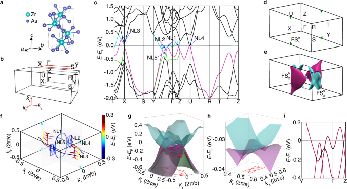
a Crystal structure of ZrAs2. b First Brillouin zone (surface and bulk) of ZrAs2, highlighting its high symmetry points and the projection of the (001) surface. c Electronic band structure of ZrAs2 obtained using first-principles calculations (without considering spin-orbit coupling) along high-symmetry lines. d, e Three-dimensional Fermi surface of ZrAs2 displaying two hole-like (\({{{{\rm{FS}}}}}_{1}^{{{{\rm{h}}}}}\) and \({{{{\rm{FS}}}}}_{2}^{{{{\rm{h}}}}}\)) and one electron-like (\({{{{\rm{FS}}}}}_{1}^{{{{\rm{e}}}}}\)) pockets. The color code corresponds to the bands shown in panel (c). f Nodal loops in the kx-ky-kz space formed by the band crossings between green, magenta, and cyan bands in panels (c, g, h). Three-dimensional visualization of the electronic band crossings and the nodal lines or loops (red lines) within the \({k}_{z}=0\) (panel g) and \({k}_{y}=0\) planes near the U point (panel h). Bands are shown using the same color as in (c). The projection in E-EF = 0 plane indicates the location of the nodes in momentum space. i Enlarged view of the band structure along the Y → Γ → Z direction, contrasting bands with (red) and without (black) spin-orbit coupling.
To experimentally confirm the nodal features within the electronic band structure, we conducted angle-resolved photoemission spectroscopy (ARPES) measurements, which directly visualize the electronic bands. In Supplementary Fig. 6, we present ARPES data alongside an ab initio energy-momentum cut along the Y → Γ→Y path. ARPES energy-momentum (E-k) cut along the \(\bar{{{{\rm{Y}}}}}-\,\bar{\Gamma }-\bar{{{{\rm{Y}}}}}\) path (Supplementary Fig. 6b) reveals two sets of band crossings: one located at \(E-{E}_{f}=\,-0.29\,{{{\rm{eV}}}}\) and another one near the Fermi level. These crossings align closely with the ab-initio calculations (Supplementary Fig. 6c), despite some bands being suppressed by matrix element effects or kz broadening. These two crossings correspond to nodal lines NL5 and NL1, respectively. The excellent agreement between ARPES and the DFT calculations provides evidence for the existence of nodal lines in ZrAs₂. It is worth mentioning that, in the presence of spin-orbit coupling, the band crossings are lifted, leading to the emergence of a gap ranging from 2 to 58 meV (depending on the specific nodal feature), as depicted in Fig. 1j. The small gaps (e.g., 10 meV and 2 meV for NL1 and NL5, respectively) fall below the ARPES energy resolution (approximately 15 meV) and, therefore, cannot be observed under the presence of the kz or extrinsic broadening and thus can be generally ignored47,48; see Supplementary Fig. 6c. Therefore, NL1 and NL5 can be effectively treated as a nodal line state under these conditions.
Having uncovered the band topology of ZrAs2, we performed systematic electrical transport measurements. For this investigation, we selected a small, uniform, needle-shaped crystal and attached four electrical contacts on the ab-plane [(001) surface] of ZrAs2 using silver epoxy; see Supplementary Information Section II and Supplementary Fig. 7 on how we determined the crystal plane prior to conducting the measurements. This configuration allows measurements of the longitudinal resistance (R) using the standard four-probe method. Figure 2a illustrates the temperature dependence of R. At elevated temperatures, R displays metallic behavior (\({dR}/{dT} > 0\)), indicative of transport being dominated by phonon-scattering49. The residual resistivity ratio of approximately 35 indicates high sample quality and a significant variation in resistivity with temperature. Remarkably, the resistance undergoes a sudden drop to zero, marking the onset of superconductivity with a Tc of 1.8 K, which is the highlight of our investigation. Notice that Zr becomes a type-I superconductor below Tc of 0.6 K, while As only becomes superconducting under very high hydrostatic pressures50,51. Therefore, the observed superconducting state ought to be intrinsic to ZrAs2. To investigate its characteristics, we probed the magnetoresistance well below Tc, at \(T=0.3\) K, while varying the magnetic field orientation, spanning from the c-axis [001] (\(\theta={0}^{o}\)) to the [100] direction (\(\theta={90}^{o}\)) of ZrAs2 (Fig. 2b). A crucial observation obtained from the magnetoresistance traces in Fig. 2b is the upper critical magnetic field (\({H}_{{{{\rm{c}}}}2}\)), corresponding to the field at which the resistance attains 50% of its normal state value. In Fig. 2c, we chart \({H}_{{{{\rm{c}}}}2}\) as a function of θ. As the magnetic field direction progresses from the out-of-plane (\(\theta={0}^{o}\)) to in-plane (\(\theta={90}^{o}\)) orientation with respect to the (001)-plane of ZrAs2, the transition to the (field-induced) normal state systematically shifts to higher fields, with the maximum \({{\mu }_{0}H}_{{{{\rm{c}}}}2}\)(\(\theta\)) recorded at \(\theta={90}^{o}\) (Fig. 3c). The in-plane \({\mu }_{0}{H}_{{{{\rm{c}}}}2}\) is determined to be approximately 3.66 T, which is 11% larger than the weak coupling Pauli (or Clogston–Chandrasekhar) paramagnetic limit, \({{\mu }_{0}H}_{p}=1.84\times\)Tc T/K = 3.3 T for BCS superconductors52,53. This observation underscores a superconducting anisotropy, captured by the Tinkham formula governing the angular dependence of \({H}_{{{{\rm{c}}}}2}\) for a two-dimensional superconductor54: \(\left|\frac{{H}_{{{{\rm{c}}}}2}\left(\theta \right){{{\rm{cos}}}} \theta }{{H}_{{{{\rm{c}}}}2,\perp }}\right|+{\left(\frac{{H}_{{{{\rm{c}}}}2}\left(\theta \right){{{\rm{sin}}}} \theta }{{H}_{{{{\rm{c}}}}2,{{||}}}}\right)}^{2}=1.\) Here, \({{\mu }_{0}H}_{{{{\rm{c}}}}2,\perp }\) and \({{\mu }_{0}H}_{{{{\rm{c}}}}2,{{{\rm{||}}}}}\) represent the upper critical magnetic fields for fields perpendicular and parallel to the sample plane, respectively. As depicted in Fig. 2c, our data aligns well with the Tinkham formula while revealing deviations (for near \(\theta=90^\circ\)) from the Ginzburg-Landau anisotropic mass model52, which characterizes the angular dependence of \({{\mu }_{0}H}_{{{{\rm{c}}}}2}\) for a three-dimensional superconductor as: \({\left(\frac{{H}_{c2}\left(\theta \right){{{\rm{cos}}}} \theta }{{H}_{{{{\rm{c}}}}2,\perp }}\right)}^{2}+{\left(\frac{{H}_{c2}\left(\theta \right)\sin \theta }{{H}_{{{{\rm{c}}}}2,{||}}}\right)}^{2}=1\). The conformity to the Tinkham formula is consistent with our observation of the (slight) violation of the Pauli limit. The \(\theta\)-dependent measurements thus suggest that the superconductivity in ZrAs2 is in the two-dimensional limit.
Fig. 2: Superconducting instability in ZrAs2.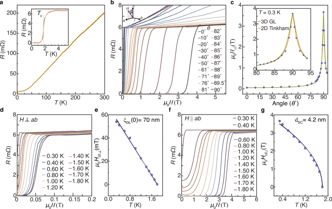
a Four-probe resistance (R) of a small ZrAs2 single-crystal, exhibiting metallic behavior as a function of the temperature (T) before transitioning to a superconducting state at Tc \(\simeq\)1.8 K. The inset depicts a magnified image of the resistance as a function of the temperature trace near Tc. b Resistance at \(T\simeq 0.3\) K as a function of the magnetic field for different out-of-the-plane rotation angles (\(\theta\)). The inset illustrates the direction of rotation, where \(\theta\) represents the angle between the out-of-plane magnetic field and the c-axis of the crystal. c \(\theta\)-dependence of the upper critical magnetic field (\({\mu }_{0}{H}_{{{{\rm{c}}}}2}\)), defined as the field at which the resistance becomes half of its value in the normal state just above the transition. The orange and green curves represent the values expected from the Tinkham formula for a two-dimensional superconductor and the three-dimensional Ginzburg-Landau anisotropic mass model, respectively, considering the observed out-of-plane upper critical field (\({\mu }_{0}{H}_{{{{\rm{c}}}}2,\perp }=0.056\) T) and in-plane upper critical field (\({{\mu }_{0}H}_{{{{\rm{c}}}}2,{{{\rm{||}}}}}=3.66\) T). Inset: A magnified view of the same data near \(\theta={90}^{{{{\rm{o}}}}}\). The data show excellent agreement with the Tinkham formula while deviating from the three-dimensional Ginzburg-Landau anisotropic mass model, particularly near \(\theta={90}^{{{{\rm{o}}}}}\). d Resistance as a function of the out-of-plane magnetic field for different temperatures. e Temperature dependence of \({\mu }_{0}{H}_{{{{\rm{c}}}}2,\perp }\), displaying a linear dependence on T close to Tc. The dark blue line represents a fit to the Ginzburg-Landau model for two-dimensional superconductors, yielding an in-plane coherence length of \({\xi }_{{{{\rm{GL}}}}}\left(0\right)\simeq 70\) nm. f Resistance as a function of the out-of-plane magnetic field for different temperatures. g Temperature dependence of \({{\mu }_{0}H}_{{{{\rm{c}}}}2,{{{\rm{||}}}}}\). The dark blue line depicts a fit to the Ginzburg-Landau model for two-dimensional superconductors, yielding a superconducting thickness of \({d}_{{{{\rm{SC}}}}}\simeq 4.2\) nm.
Fig. 3: Observation of the Berezinskii–Kosterlitz–Thouless (BKT) transition.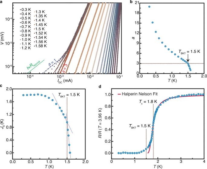
a Voltage (V)-current (I) characteristics acquired in the low-current regime, in a logarithmic scale, and for different temperatures. The red, blue, and green dashed lines represent \({V}\propto \,{I}^{3}\), \({V}\propto {I}\), and \(V={I\; R}\)Normal, respectively. b Temperature dependence of the exponent \(a(T)=1+\pi {J}_{S}(T)/{T}\) extracted from fitting the V-I data to \(V\propto {I}^{a\left(T\right)}\). The BKT transition is characterized by \(\pi {J}_{S}({T}_{{{{\rm{BKT}}}}})/{T}_{{{{\rm{BKT}}}}}=2\), leading to \(a({T}_{{{{\rm{BKT}}}}})\,=\,3\), the relation that defines \({T}_{{{{\rm{BKT}}}}}\). The horizontal dashed line indicates the value \(a=3\). \(a(T)\) as a function of \(T\) clearly reveals the BKT transition with \({T}_{{{{\rm{BKT}}}}}\simeq 1.5\) K. c Temperature dependence of the superfluid stiffness, \({J}_{S}.\,{J}_{S}\) drops near \({T}_{{{{\rm{c}}}}}\), as expected from the BCS theory. Above \({T}_{{{{\rm{BKT}}}}}\simeq 1.5\) K, the \({J}_{S}\) decreases more rapidly with increasing T, as shown by the violet dashed lines serving as guides to the eye. d Temperature dependence of the resistance (blue circles), fitted to the Halperin–Nelson theory using the parameters \({T}_{{{{\rm{BKT}}}}}=1.5\) K and \({T}_{{{{\rm{c}}}}}=1.8\) K. The Red curve represents the best fit.
To gain further insights into the superconducting transition, we conducted systematic temperature-dependent measurements in Fig. 2d and e provide a visual representation of the acquired results when the magnetic field was applied perpendicularly to the ZrAs2 (001) plane. It is worth noting that the superconducting transition progressively shifts to lower magnetic fields with increasing temperature. This evolution of the temperature-dependent out-of-plane upper critical magnetic fields (\({\mu }_{0}{H}_{{{{\rm{c}}}}2,\perp }\)) is summarized in Fig. 2e. Given that the angular dependence of \({\mu }_{0}{H}_{{{{\rm{c}}}}2}(\theta )\) can be described by a two-dimensional superconductivity model, it is anticipated that \({\mu }_{0}{H}_{{{{\rm{c}}}}2,\perp }\) would exhibit a linear relationship with temperature close to Tc as given by the standard Ginzburg-Landau model for two-dimensional superconductors54: \({{\mu }_{0}H}_{{{{\rm{c}}}}2,\perp }\left(T\right)=\,\frac{{\varPhi }_{0}}{2\pi {\xi }_{{{{\rm{GL}}}}}{(0)}^{2}}(1-\frac{T}{{T}_{c}})\). Here \({\xi }_{{{{\rm{GL}}}}}(0)\) stands for the zero-temperature in-plane coherence length, \({\varPhi }_{0}\) is the magnetic flux quantum, and Tc is the critical temperature. Indeed, near Tc, \({\mu }_{0}{H}_{{{{\rm{c}}}}2,\perp }\) displays linear behavior as a function of T before dropping to zero at Tc as expected for two-dimensional superconductivity. By fitting the data, we estimate \({\xi }_{{{{\rm{GL}}}}}\left(0\right)\) to be 70 nm. We also examined the temperature-dependent superconducting transition with the magnetic field applied parallel to the sample ab plane. Figure 2f shows the corresponding traces, and Fig. 2f summarizes the result, illustrating the in-plane upper critical field \({H}_{{{{\rm{c}}}}2,{||}}\) as a function of temperature. Akin to \({{\mu }_{0}H}_{{{{\rm{c}}}}2,\perp }\left(T\right)\), \({{\mu }_{0}H}_{{{{\rm{c}}}}2,{||}}\left(T\right)\) can be fitted to the standard Ginzburg-Landau model for two-dimensional superconductors54: \({{\mu }_{0}H}_{{{{\rm{c}}}}2,{||}}\left(T\right)=\,\frac{{\varPhi }_{0}\sqrt{3}}{\pi {\xi }_{{{{\rm{GL}}}}}(0){d}_{{{{\rm{sc}}}}}}{(1-\frac{T}{{T}_{c}})}^{1/2}\) near Tc. From this fit, we extract a superconducting thickness \({d}_{{SC}}\approx 4.2\) nm, which is approximately 17 times smaller than \({\xi }_{{{{\rm{GL}}}}}\left(0\right)\). Despite the good agreement with the fits to two-dimensional superconductivity, it should be noted that \({d}_{{SC}}\) is much smaller (by at least 4 orders of magnitude) than the sample thickness but at least 4 times larger than the c-axis lattice constant of ZrAs2, suggesting that its superconductivity could be confined to just 4 unit-cells at ZrAs2 (001) plane.
The apparent two-dimensional superconductivity in ZrAs2 cannot be directly attributed to the dimensionality of the bulk Fermi surface, which we directly probed through our quantum oscillatory experiments as depicted in Supplementary Figs. 4 and 5. The magnetoresistance traces displayed in Supplementary Figs. 4 and 5 reveal distinct \(1/{\mu }_{0}H\)-periodic quantum oscillations (or the Shubnikov-de Haas effect). By analyzing the quantum oscillatory data (detailed in Supplementary Figs. 4 and 5, with a discussion in Supplementary Information Section I), we observe that while the quantum oscillatory frequencies (f2 and f3) display dependence on magnetic field orientation, neither conforms to the \(1/\cos \theta\) dependency characteristic of two-dimensional Fermi surfaces. This observation implies that the carriers arising from these bulk Fermi surfaces are unlikely to contribute to the Cooper pairing mechanism. As discussed below, we therefore argue that the driving factor behind the superconductivity in ZrAs2 is associated with paired charge carriers on the surface state of the ab plane.
Given that ZrAs2 demonstrates a superconducting transition in resistivity measurements, one would anticipate the appearance of the Meissner effect. However, testing of multiple samples revealed that, despite the observable superconducting transition in the resistivity, the Meissner effect is absent down to 1.69 K (as shown in Supplementary Information Section III and Supplementary Fig. 8). Furthermore, as detailed in Supplementary Information Section IV and Supplementary Fig. 9, our muon spin relaxation (μSR) measurements in ZrAs2 show no signature of a bulk superconducting state down to 0.04 K. The most likely explanation is that the superconductivity is confined to the surfaces of ZrAs2. Magnetic DC susceptibility and μSR measurements require a large sample volume for the detection of the diamagnetic response associated with a superconducting transition. Consequently, if only the surface would superconduct and not the bulk of the material, such a state will not be captured by these techniques. This distinction likely explains why we did not observe signatures for superconductivity in ZrAs₂ from the magnetic susceptibility or μSR measurements since the superconductivity in this material is limited to its surface with the non-superconducting bulk contribution dominating the magnetic susceptibility and the μSR signals. Notably, the angular dependence of the \({\mu }_{0}\)Hc2 (\(\theta\)) aligns with the possibility of superconductivity emerging solely in the ab plane of the orthorhombic crystal. Such a surface-confined superconducting state is expected to exhibit behavior characteristic of the two-dimensional limit, which is precisely what we observe in our measurements of \({\mu }_{0}\)Hc2 (\(\theta\)), \({{\mu }_{0}H}_{{{{\rm{c}}}}2,\perp }\left(T\right)\), and \({\mu }_{0}{H}_{{{{\rm{c}}}}2,{||}}\left(T\right)\). It is also worth noting that a surface superconductor like ZrAs2 is different from quasi-2D superconductors like YBa₂Cu₃O₇₋δ, which exhibit superconductivity in all layers, i.e., in the bulk. Therefore, its superconductivity can be detected through magnetic susceptibility and μSR measurements.
The observation of two-dimensional superconductivity in a bulk single crystal sample lacking a quasi-two-dimensional Fermi surface, coupled with the absence of bulk superconductivity, strongly suggests that the pairing mechanism is exclusively driven by carriers on the surface state. This unique surface superconductivity fundamentally differs from three-dimensional superconductors, as it should give rise to the spontaneous emergence of vortices due to the Berezinskii–Kosterlitz–Thouless (BKT) transition in two-dimensions55,56. Through an examination of the voltage (V)- current (I) relationship obtained via electrical transport measurements across various temperatures, we uncover clear signatures of a BKT transition that reinforce the notion of the surface-confined nature of the superconducting state. As illustrated by Fig. 3a, at low temperatures, distinctive nonlinearities manifest in the V(I) characteristics, conforming to a temperature-dependent power law57: \(V\propto {I}^{a\left(T\right)}\), where \(a(T)=1+\pi {J}_{S}(T)/T\), and \({J}_{S}\) represents the superfluid stiffness. The precise occurrence of the BKT transition is determined by the condition \(\pi {J}_{S}({T}_{{{{\rm{BKT}}}}})/{T}_{{{{\rm{BKT}}}}}=2\), yielding \(a({T}_{{{{\rm{BKT}}}}})=3\) and thereby defining the value of \({T}_{{{{\rm{BKT}}}}}\). We identified such behavior in the V(I) characteristics, which are plotted in Fig. 3a and b, where a cubic power law is evident for \(T\simeq 1.5\) K. Note that for the BKT transition in an infinite and homogeneous sample, a universal jump of \(a(T)\) is anticipated at the BKT temperature (TBKT), transitioning from \(a(T > {T}_{{{{\rm{BKT}}}}})=1\) to \(a(T . However, in practice, all samples inherently possess inhomogeneities or defects and are of a finite size. Consequently, the discontinuity in \(a(T)\) at \({T}_{{{{\rm{BKT}}}}}\) is anticipated to broaden but must occur at a temperature between \(T={T}_{{{{\rm{c}}}}}\) and \(T={T}_{{{{\rm{BKT}}}}}\)57. In ZrAs2, we find that \(a(T)\) decreases rather sharply with increasing temperature and falls to 1 within 0.08 K of \({T}_{{{{\rm{BKT}}}}}\). Such a dramatic change in \(a(T)\) is consistent with what one expects from the BKT transition.
For a consistency check, we also plot the superfluid stiffness \({J}_{S}\,(T)\) obtained from \(\frac{T}{\pi }\left(a\left(T\right)-1\right)\) in Fig. 3c. We find that at low temperatures, \({J}_{S}\,(T)\) saturates, and elevated temperatures, \({J}_{S}\,(T)\) becomes smoothly suppressed as quasiparticles emerge when the temperature is raised, as qualitatively expected from the BCS theory; see Supplementary Information Section VI and Supplementary Fig. 4 for the BCS fitting results. Importantly, above \({T}_{{{{\rm{BKT}}}}}\), \({J}_{S}\,(T)\) drops much rapidly as one would expect from the BKT transition. Note that the power dissipated in the sample corresponding to the traces presented in Fig. 3a is maximum 50 picowatts. Such a small power dissipation is unlikely to cause Joule heating of the sample.
Next, we scrutinized the temperature dependence of the resistance near the superconducting transition. Using the Halperin–Nelson theory58, Benfatto et al. 57 formulated the temperature dependence of the resistance for \(T\ge {T}_{{{{\rm{BKT}}}}}\) as \(\frac{R\left(T\right)}{{R}_{{{{\rm{N}}}}}}=\frac{1}{1+{A}_{{HN}}\sin {h}^{2}\left(\sqrt{{B}_{{HN}}\frac{{T}_{c}-{T}_{{BKT}}}{T-{T}_{{BKT}}}}\right)}\). Here, RN represents the normal state resistivity, BHN stands for a dimensionless constant of the order of 1, and AHN is a pre-factor. By fixing \({T}_{{{{\rm{BKT}}}}}\) at the value obtained from the V(I) characteristics, namely \({T}_{{{{\rm{BKT}}}}}=1.5\) K, we achieve a good fit to the experimental data (Fig. 3d). The good agreement with the Halperin–Nelson formula underscores that the superconducting state in ZrAs2 resembles that of a pure superconducting state, as the formula assumes a homogenous superconducting state with no broadening in \({T}_{{{{\rm{BKT}}}}}\). This observation is indeed in harmony with the high quality of the sample, as indicated by its substantial residual-resistivity ratio and the clear presence of quantum oscillatory phenomena (see Supplementary Information Section I). Importantly, it is worth emphasizing that, the BKT transition has previously been observed only in quasi-2D-layered superconductors and thin films59,60,61,62,63. Here, we argue that this work represents the first solid and complete study demonstrating the presence of superconductivity confined exclusively to the surface of any given compound.
In effect, surface superconductivity was previously claimed for CaAgP64 and its Pd-doped version, as well as for PtBi265. For CaAgP and its Pd-doped variant, point contact spectroscopy would imply strong coupled, spin-triplet chiral superconducting pairing. However, such conclusions are at odds with the very small upper critical fields measured by the same authors, frequently seen in non-uniform, filamentary superconductors66, thus suggesting that these hypotheses require additional experimental confirmation. In ref. 64, and in contrast to our data, the surface superconducting transition does not lead to a zero-resistance state, while the surface superconducting state in CaAgP is found to be easily suppressed by the application of very small fields, i.e., μ0H = 31 mT, in contrast to ZrAs2 whose planar upper critical fields exceed μ0H = 3.5 T at T = 300 mK. Notice that this is at odds with the authors’ claims of spin-triplet p-wave superconductivity in Pd doped CaAgP, based on point contact spectroscopy, which would not be subjected to the Pauli limit. It is also at odds with the authors’ claims in favor of strong coupled superconductivity, as suggested by the large ratio between the superconducting gap and the transition temperature, which the authors claim to substantially exceed the BCS ratio. As is well known for strongly correlated systems, e.g., heavy fermion superconductors, electronic correlations substantially renormalize orbital and Pauli upper critical fields towards very high values. Therefore, we find inconsistencies between their claims and observations. Notice that we also extract a large ratio between the superconducting gap \(\Delta\) and Tc, i.e., \(\Delta\)/Tc = \(2.685\), see Supplementary Information Section VI. But this is consistent with the measured upper critical fields perpendicular and along the planes that considerably exceed the Pauli limiting field μ0Hp = 1.84 \(\times \,\)Tc = 3.3 T, as one reduces the temperature towards zero (Fig. 2). As for PtBi2, the conclusion in favor of superconductivity below Tc \(\approx\) 10 K is based on the loss of the spectral weight of the Fermi arcs. Nevertheless, relatively thick exfoliated flakes from this type-I Weyl compound exhibit superconducting transitions well below 1 K, according to transport measurements62. Therefore, further work is required to elucidate the seemingly contradictory behavior of these superconductors. In contrast, our work on ZrAs2 reveals a clear zero-resistance state, high planar upper critical fields, and a BKT-like superconducting transition, all in the absence of any evidence for bulk superconductivity, clearly suggesting a surface superconducting state.
The observation of surface-confined superconductivity in ZrAs2 prompts us to explore the potential mechanisms that could stabilize such pairing in the surface state. To this end, we investigated the surface-projected Fermi surface and band structure. The ab initio calculations (incorporating spin-orbit coupling) of the surface state projected onto the (001) plane, where we observe the superconducting state, show termination-dependent surface state contribution. We consider the termination which matches our experimental data (see supplementary Information Section VIII and Supplementary Figs. 11 and 12). The calculations reveal a vHs located at the \(\bar{{{{\rm{X}}}}}\) point in the band corresponding to the surface state at approximately 65 meV below the Fermi level (see Fig. 4a, b). This saddle point is characterized by the crossing of the surface states at a constant energy contour (Fig. 4c). This observation is also evident in the three-dimensional view of the band structure of the surface state within the kx-ky plane, around the \(\bar{{{{\rm{X}}}}}\) point, as depicted in Fig. 4c. The saddle point, or vHs, results from the intersection of two symmetric pockets in the constant energy contours at the high symmetry \(\bar{{{{\rm{X}}}}}\)-point.
Fig. 4: Surface van Hove singularity near the Fermi energy.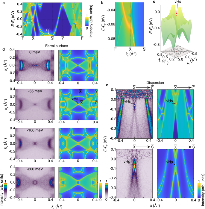
a Ab-initio calculations (considering spin-orbit coupling) of the band structure projected onto the (001) surface, revealing the presence of surface states (SS), marked with arrows, and a van Hove singularity (vHs) at the \(\bar{{{{\rm{X}}}}}\) point. b Magnified view of the saddle point at the \(\bar{{{{\rm{X}}}}}\) point, marked with a red circle in panel (a). c Three-dimensional view of the surface state dispersion near the vHs at the \(\bar{{{{\rm{X}}}}}\) point on the kx-ky plane with kz fixed at 0 Å. d Angle-resolved photoemission spectra (left column) and corresponding ab-initio calculations (considering spin-orbit coupling) illustrating the surface-projected constant energy contours at Eb = 0 eV,– 65 meV (where the vHs is located), − 100 meV, and 200 meV. For convenience, the coordinates of the \(\bar{{{{\rm{X}}}}}\) point are chosen to correspond to the (0, 0) coordinates. The photoemission spectroscopy results align with the calculated constant energy contours. The black arrow on the Fermi surface of the surface state indicates the location of the vHs, identified by the intersections among surface states. e Energy-momentum slices along the \(\bar{\Gamma }-\,\bar{{{{\rm{X}}}}}-\,\bar{\Gamma }\) and \(\bar{{{{\rm{S}}}}}-\,\bar{{{{\rm{X}}}}}-\,\bar{{{{\rm{S}}}}}\) directions acquired with photoemission spectroscopy (left column) and the (001) surface-projected calculation (right). The surface states (marked by white dashed parabolic bands) exhibit electron-like dispersion along \(\bar{\Gamma }-\,\bar{{{{\rm{X}}}}}-\,\bar{\Gamma }\) and hole-like dispersion along \(\bar{{{{\rm{S}}}}}-\,\bar{{{{\rm{X}}}}}-\,\bar{{{{\rm{S}}}}}\) the direction, forming a saddle point (marked by the black arrow) at the \(\bar{{{{\rm{X}}}}}\) point. For each binding energy, the energy-momentum cuts (panel e) are normalized at each binding energy to highlight band intensities near the Fermi level. The units in all the color bars shown are arbitrary units.
To experimentally probe the vHs around the \(\bar{{{{\rm{X}}}}}\) point, we conducted further ARPES measurements. Figure 4d illustrates the evolution of the constant energy contours across consecutive energy slices; the left panels display the experimental results, while the right panels depict the corresponding ab initio calculations. As observed in Fig. 4d, two symmetry-related butterfly-wing-shaped states are separate at the Fermi level, with the apex of each pocket lying along the \(\bar{\Gamma }-\,\bar{{{{\rm{X}}}}}\) direction. As the energy is lowered to − 65 meV, the two states converge, ultimately leading to an intra-band intersection at the \(\bar{{{{\rm{X}}}}}\) point, thus forming a vHs. Further changes in energy towards − 100 meV and − 150 meV reveal butterfly-like features and their intersecting section near the \(\bar{{{{\rm{X}}}}}\) point becomes hole-like. The presence of vHs in the surface state is also evident in the energy-momentum slices along the \(\bar{\Gamma }-\,\bar{{{{\rm{X}}}}}-\,\bar{\Gamma }\) and \(\bar{{{{\rm{S}}}}}-\,\bar{{{{\rm{X}}}}}-\,\bar{{{{\rm{S}}}}}\) directions. Figure 4e illustrates these results, showcasing the energy-momentum dispersion spectra on the (001) surface projected ab initio calculations. Notably, the (001) surface state displays an electron-like dispersion along the \(\bar{\Gamma }-\,\bar{{{{\rm{X}}}}}-\,\bar{\Gamma }\) direction and a hole-like dispersion along the \(\bar{{{{\rm{S}}}}}-\,\bar{{{{\rm{X}}}}}-\,\bar{{{{\rm{S}}}}}\) direction, thus highlighting the formation of a saddle point at the \(\bar{{{{\rm{X}}}}}\) point. Therefore, our ARPES spectra combined with ab initio calculations unveil a vHs around the \(\bar{{{{\rm{X}}}}}\) point in the electronic surface bands of the (001) plane, precisely where we observe the two-dimensional superconducting state.
To further distinguish between surface and bulk contributions to the observed vHs, we performed a detailed photon-energy-dependent ARPES study. Figure 5 summarizes our results. Our analysis reveals that at the binding energy \({E}_{{{{\rm{B}}}}}={E}_{{{{\rm{vHs}}}}}\), the contour of the vHs state near the \(\bar{{{{\rm{X}}}}}\) point remains consistent across the photon energy range studied (35–55 eV), as illustrated in Fig. 5f. Furthermore, the peaks in the momentum distribution curves at\({E}_{{{{\rm{B}}}}}={E}_{{{{\rm{vHs}}}}}-0.1\) eV, corresponding to the hole dispersion of the VHS state along the \(\bar{{{{\rm{S}}}}}\)-\(\bar{{{{\rm{X}}}}}\)-\(\bar{{{{\rm{S}}}}}\) direction, show no variation with photon energy, as illustrated in Fig. 5f. In contrast, the bulk state near the \(\bar{\Gamma }\) point shows significant variation with photon energy, underscoring the distinct behavior inherent to bulk states. This absence of photon energy dependence for the vHs state suggests that it results from a surface state, as surface states are independent of photon energy, unlike bulk states. We refer the readers Supplementary Fig. 13a–c for additional results supporting that the vHs is formed by the surface state.
Fig. 5: Photon energy dependence of the van Hove singularity (vHs) state at the \(\bar{{{{\bf{X}}}}}\) point.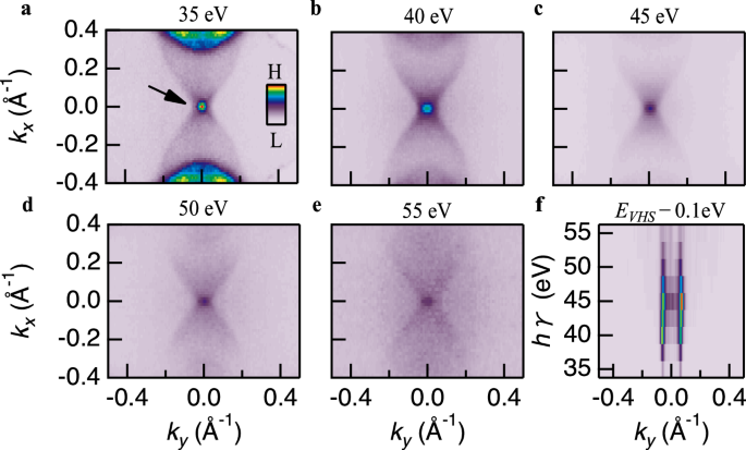
a–e Constant energy contours at the fixed energy of the vHs (EvHs), measured at photon energies of 35, 40, 45, 50, and 55 eV, respectively. Note that the maps are symmetrized with respect to \({k}_{x}=0\). f Photon energy dependence of the momentum distribution curves measured at EvHs – 0.1 eV along the \(\bar{{{{\rm{S}}}}}\)-\(\bar{{{{\rm{X}}}}}\)-\(\bar{{{{\rm{S}}}}}\) direction. The contour of the vHs state remains unchanged across different photon energies, demonstrating its surface state nature. H and L in the color bar shown in panel (a) denote high and low intensities, respectively.
The presence of a vHs in the kx-ky-plane within the first Brillouin zone indicates an enhanced density of states at − 65 meV, which is slightly below the Fermi energy (see Supplementary Figs. 14 for the ARPES results and 15 for the ab-initio calculations) within that plane. Supplementary Fig. 14 presents energy distribution curves along two orthogonal directions passing through the \(\bar{{{{\rm{X}}}}}\) point. We find that the peak observed at the top band along the \(\bar{S}-\,\bar{X}-\,\bar{S}\) direction aligns with the bottom of the band along the \(\bar{\Gamma }-\,\bar{X}-\,\bar{\Gamma }\) path, forming a two-dimensional saddle point. This saddle point in the surface state dispersion naturally results in vHs, owing to the inevitable divergence of the density of states at the saddle point of a two-dimensional electronic state67,68. The corresponding increased density of states, which can be further explored via future tunneling measurements, has the potential to induce electronic order, such as superconductivity. Our transport experiments, presented in Figs. 2 and 3, reveal that the superconducting state is confined within the ab-plane, which is directly connected with the kx-ky-plane in the first Brillouin zone where the vHs is located (Fig. 4). Hence, it is likely that the vHs, and concomitant enhanced density of states, play a pivotal role in stabilizing the superconducting state on the same surface.