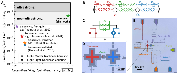
Quarton coupler circuit
Superconducting circuits is a leading platform for the study and control of light-matter interaction26,27. By exploiting the nonlinear kinetic inductance of the Josephson junction (JJ) to make quantum oscillators with nonlinear energy levels, high coherence artificial atoms or qubits can be realized. We use here a common type of superconducting qubit, known as the transmon28, which can be understood as a microwave resonator with added self-Kerr nonlinearity (K
$${\hat{H}}_{{{{\rm{transmon}}}}}={\omega }_{b}{\hat{b}}^{{{\dagger}} }\hat{b}+\frac{K}{2}{\hat{b}}^{{{\dagger}} 2}{\hat{b}}^{2}+\cdots \approx \frac{{\omega }_{b}}{2}{\hat{\sigma }}_{z},$$
(3)
The key insight is that since adding a self-Kerr of K turns a linear resonator (photonic) mode into a qubit (atomic) mode, then removing K linearizes a transmon qubit into a resonator. This is achieved using the quarton coupler we proposed in ref. 25, which can induce an opposite-signed (positive) self-Kerr to transmons while facilitating large cross-Kerr between them. This “quartonic” approach allows us to achieve large cross-Kerr χ without causing a large self-Kerr K that would otherwise compromise the linearity of the photon mode. We contrast our approach with the state-of-the-art in Fig. 1A which shows the parameter landscape of light-matter nonlinear coupling (including 1 additional case of light-light nonlinear coupling24) with 4-wave-mixing Kerr effect, wherein we use calculated Ka when not provided19,29. To the best of our knowledge, all previous experimental cross-Kerr demonstrations19,24,29,30 are limited to ∣χ∣/max(ωa, ωb) O(10−2) and a trade-off appears where larger nonlinear coupling is accompanied by disproportionately larger self-nonlinearity (decreasing \(| \chi | /\sqrt{| {K}_{a}{K}_{b}| }\)). Existing demonstrations are also limited to \(| \chi | /\sqrt{| {K}_{a}{K}_{b}| } \sim O(1)\), as expected when cross-Kerr interactions are dominated by first-order effects which satisfy \(| \chi | /\sqrt{| {K}_{a}{K}_{b}| }=2\)31. This helps explain the difficulty in reaching large light-matter cross-Kerr, given that resonator Ka needs to be minimized while the qubit Kb is typically limited by noise trade-offs28, and the inability for past works to exceed \(| \chi | /\sqrt{| {K}_{a}{K}_{b}| }\approx 2\). Reaching large light-light cross-Kerr is even more difficult since both Ka, Kb must be limited. We emphasize that the much larger \(| \chi | /\sqrt{| {K}_{a}{K}_{b}| }\gg 2\) demonstrated with the quarton coupler in this work is indicative of its unique operating principles that allow for simultaneous large cross-Kerr and self-Kerr cancellation25.
The circuit realized in this work, shown in Fig. 1C, consists of two transmons (red, blue) galvanically coupled by a gradiometric quarton coupler (green). The gradiometric circuit topology is inspired by other works32,33. The circuit’s potential energy can be written in terms of Josephson energies EJ and the node superconducting phases ϕa, ϕb:
$$U= -{E}_{Ja}\cos (\frac{{\tilde{\phi }}_{s}}{2})\cos ({\phi }_{a})-{E}_{Jb}\cos ({\phi }_{b})\\ -3{E}_{J}\cos (\frac{{\phi }_{a}-{\phi }_{b}}{3})\\ -\alpha {E}_{J}\cos ({\tilde{\phi }}_{q{{\Sigma }}})\cos ({\phi }_{a}-{\phi }_{b}),$$
(4)
where we have assumed that the two nominally identical loops of the gradiometric quarton are identically flux-biased. The gradiometric quarton then behaves as a quarton with \({\tilde{\phi }}_{q{{\Sigma }}}\) flux tunable α, which varies its ratio of linear coupling, \({({\phi }_{a}-{\phi }_{b})}^{2}\), to nonlinear coupling, \({({\phi }_{a}-{\phi }_{b})}^{4}\)25. At \(\alpha \cos ({\tilde{\phi }}_{q{{\Sigma }}})=-1/3\), the quarton coupling potential \(\frac{{E}_{Q}}{24}{({\phi }_{a}-{\phi }_{b})}^{4}+\ldots \,\) is to leading order quartic with effective Josephson energy \({E}_{Q}=\frac{8}{27}{E}_{J}\).
The behavior of this circuit can be understood with a spring-mass analogue as shown in Fig. 1B, where we treat the two node phases ϕa, ϕb as position coordinates, and the transmon JJs act as slightly nonlinear springs with spring constant EJ. Keeping terms up to O(ϕ4), the quarton acts as a purely nonlinear coupling spring with potential energy \(\frac{{E}_{Q}}{24}{({\phi }_{a}-{\phi }_{b})}^{4}\). This allows cancellation of the \(-\frac{{E}_{Ja}}{24}{\phi }_{a}^{4}\) self-nonlinearity of the ϕa mode (if EQ ≈ EJa) while creating a strong \({\phi }_{a}^{2}{\phi }_{b}^{2}\) nonlinear coupling between the two modes. Writing the ϕ operators in the Fock basis, one can see that this \({\phi }_{a}^{2}{\phi }_{b}^{2}\) coupling leads to a non-perturbative cross-Kerr term \(\propto {\hat{a}}^{{{\dagger}} }\hat{a}{\hat{b}}^{{{\dagger}} }\hat{b}\).
A false-colored micrograph of our device is shown in Fig. 1E, with a close-up of the two transmons in Fig. 1D. Transmon A, on the left, will be linearized into a light-like mode with near zero self-Kerr anharmonicity, while transmon B, on the right, will remain a nonlinear qubit or matter-like mode. Both transmons have drive lines and Purcell-protected34 readout resonators labeled A and B, which are capacitively coupled to transmons A and B, respectively. The chip also includes a local flux-bias line to tune the SQUID bias (\({\tilde{\phi }}_{s}\)) in transmon B, and the chip package has a global coil to bias the gradiometric quarton coupler. See “Methods” for more details about the experimental setup.
In addition to the quarton and SQUID loops, the upper and lower ground plane around the circuit form two loops with the JJs of the circuit (see Fig. 1D). Symmetric flux in these loops produces an unimportant screening current in the ground plane, while asymmetric flux in these loops (\({\tilde{\phi }}_{g{{\Delta }}}\)) will bias the junctions. We calibrate the local and global flux bias such that \({\tilde{\phi }}_{g{{\Delta }}}\approx 0\), so that only the SQUID (\({\tilde{\phi }}_{s}\)) and quarton (\({\tilde{\phi }}_{q{{\Sigma }}}\)) are biased (see Supplementary Note 1 for the calibration procedure).
Note that when the transmons are strongly cross-Kerr coupled, i.e. \(\chi {\hat{a}}^{{{\dagger}} }\hat{a}{\hat{b}}^{{{\dagger}} }\hat{b}\) with ∣χ∣ ≫ 0, the device exhibits an unusual phenomenon where both resonators can be used to readout either transmon. This is because the capacitive coupling g of transmon A(B) to its Δ frequency-detuned resonator A(B) hybridizes their modes, this can be approximated as \(\hat{a}(\hat{b})\to \hat{a}(\hat{b})+\frac{g}{{{\Delta }}}{\hat{a}}_{ro}({\hat{b}}_{ro})\) where \({\hat{a}}_{ro}({\hat{b}}_{ro})\) are annihilation operators of readout resonator A(B). The hybridization imparts the usual dispersive shifts, \({\chi }_{d,a}{\hat{a}}^{{{\dagger}} }\hat{a}{\hat{a}}_{ro}^{{{\dagger}} }{\hat{a}}_{ro}\) and \({\chi }_{d,b}{\hat{b}}^{{{\dagger}} }\hat{b}{\hat{b}}_{ro}^{{{\dagger}} }{\hat{b}}_{ro}\), but also an additional non-dispersive cross-Kerr χn with approximately:
$$\begin{array}{rlr}&\chi {\hat{a}}^{{{\dagger}} }\hat{a}{\hat{b}}^{{{\dagger}} }\hat{b}&\\ \to &\chi ({\hat{a}}^{{{\dagger}} }+\frac{g}{{{\Delta }}}{\hat{a}}_{ro}^{{{\dagger}} })(\hat{a}+\frac{g}{{{\Delta }}}{\hat{a}}_{ro})({\hat{b}}^{{{\dagger}} }+\frac{g}{{{\Delta }}}{\hat{b}}_{ro}^{{{\dagger}} })(\hat{b}+\frac{g}{{{\Delta }}}{\hat{b}}_{ro})\\=&\chi {\hat{a}}^{{{\dagger}} }\hat{a}{\hat{b}}^{{{\dagger}} }\hat{b}+{\chi }_{n}{\hat{a}}^{{{\dagger}} }\hat{a}{\hat{b}}_{ro}^{{{\dagger}} }{\hat{b}}_{ro}+{\chi }_{n}{\hat{b}}^{{{\dagger}} }\hat{b}{\hat{a}}_{ro}^{{{\dagger}} }{\hat{a}}_{ro}+\ldots \end{array}$$
(5)
Unlike the usual dispersive shift which for a transmon is proportional to its self-Kerr28 (χd,a(b) ∝ Ka(b)) and thus vanishes to first-order when the transmon is linearized (K ≈ 0), the non-dispersive χn is independent of transmon self-Kerrs and can thus be leveraged to readout linearized transmons.
Spectroscopy
We obtain the circuit’s eigenenergy spectrum as a function of quarton flux bias (Fig. 2A) by performing standard two-tone spectroscopy35 while sweeping Ibias (a proxy for quarton flux bias \({\tilde{\phi }}_{q{{\Sigma }}}\), see Supplementary Note 1 for details). Since transmon B is designed to have a higher frequency, we apply the drive through transmon B’s drive line (Fig. 2C) when performing spectroscopy at high frequency. For lower frequency spectroscopy, we instead drive transmon A, which is designed with a lower frequency (Fig. 2D). In both cases we use resonator B for readout because resonator A (at 6.837 GHz) is accidentally near-resonant with transitions at certain Ibias. Figure 2A reveals several transition frequencies (labeled \({f}_{{n}_{A}{n}_{B}}\) on the plot by the excitation number in transmon A(B) denoted nA(B)) of our system. By numerically solving for the eigenenergies of the circuit and fitting the Josephson energies of each JJ as free parameters (see Supplementary Note 2 for details), we obtain good agreement with the spectroscopy results (gray dashed lines).
Fig. 2: Transmon self-Kerr tuning via quarton coupler flux bias.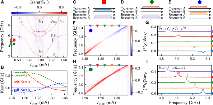
A Two-tone spectroscopy of the device with theory fit (grey dashed) overlaid. B Self- and cross-Kerr of transmons A and B at different quarton flux bias, extracted from the theory fit. Transmon A reaches zero self-Kerr at approximately Ibias = 1.285 mA. C–E Pulse sequences for two-tone spectroscopy, labeled by colored shapes. F–I High power two-tone spectroscopy near zero self-Kerr (Ibias = 1.285 mA) with pulse sequences E (for F, G) and D (for H, I). Clear signature of linearization can be observed, with peaks converging in both spectroscopies and the dispersive shift changing signs in panel (F). Panels G, I display respective line-cuts of F, H (at Ibias labeled by colored triangles), where single photon f0→1 and multi-photon f0→2/2 transitions are visible. The phase of successive line-cuts are plotted with a constant offset for visual clarity.
From the theory fit, we compute expected self- and cross-Kerrs as shown in Fig. 2B. Around the bias point Ibias = 1.285 mA, the model predicts the desired nonlinear light-matter coupling properties with near-zero self-Kerr for transmon A, non-zero self-Kerr for transmon B, and a large cross-Kerr between them. We also identify bias points such as Ibias = 1.224 mA where both transmons behave like large self-Kerr qubits, whose extremely large cross-Kerr coupling is ideal for matter-matter nonlinear coupling (also known as ZZ9 or Ising36 or longitudinal interaction37: \(\frac{\chi }{4}{\hat{\sigma }}_{z,a}{\hat{\sigma }}_{z,b}\)).
In Fig. 2F–I, we zoom in and more closely examine the flux bias near Ibias = 1.285 mA where transmon A is linearized. We perform standard high-power two-tone spectroscopy so the multi-photon transitions that reveal transmon anharmonicity can be excited35. In Fig. 2F, we drive transmon A and resonantly probe the dispersively-coupled resonator A (see Fig. 2E). We observe a clear sign change in readout phase indicating a corresponding sign change in the underying dispersive shift between resonator A and transmon A. This is expected as a resonator’s dispersive shift with a transmon (when Δ ≫ K) is directly proportional to the transmon’s self-Kerr28 (χd ∝ K), and we also observe a concurrent change in self-Kerr anharmonicity, most clearly-observed in Fig. 2G where we plot the line-cuts of Fig. 2F with constant phase offsets. Here, we see higher-order transition peaks (most visibly, f0→2/2) move from above to below the f0→1 peak and converge in the middle, near the theory-predicted zero-Kerr point Ibias = 1.285 mA. At this point, the transmon A peak is almost invisible to its dispersively-coupled readout resonator A, consistent with the prediction that the dispersive shift goes to zero at linearization.
We verify that the disappearance of transmon A (in Fig. 2F) is due to its linearization by repeating high-power two-tone spectroscopy with resonator B instead (see Fig. 2D). As derived previously (see Eq. (5)), there exists a non-dispersive cross-Kerr χn between transmon A and resonator B which does not depend on transmon A’s anharmonicity Ka. As predicted, the resulting spectroscopy (Fig. 2H, I) shows the same convergence of higher-order transitions at the linearization point but has a strong transmon A signal even when it is linearized. In fact, among the Fig. 2I line-cuts, the transmon A peak is the strongest at the linearization point (green) because more energy levels can be excited (higher \(\langle {\hat{a}}^{{{\dagger}} }\hat{a}\rangle\)) for an overall larger readout shift (\({\chi }_{n}\langle {\hat{a}}^{{{\dagger}} }\hat{a}\rangle\)) on resonator B. We also see that the phase shifts in Fig. 2H, I are all positive, in agreement with the prediction of Eq. (5) that χn ∝ χ and the quartonic χ between transmon A and B is positive (see Fig. 2B). We note that this non-local, non-dispersive cross-Kerr interaction between a transmon and a spatially-separated and geometrically-uncoupled resonator may have further applications in novel readout or remote-entanglement schemes.
Near-ultrastrong light-matter nonlinear coupling
We now demonstrate near-ultrastrong nonlinear coupling between transmon B and the linearized transmon A by operating at the linearization point (Ibias = 1.285 mA) found previously. Table 1 shows the transition frequencies and coherence times of both transmons at this operating point (see Supplementary Note 3 for details). We note that transmon A has a near-zero measured self-Kerr anharmonicity of 0.76 ± 0.08 MHz, on par with or lower than other experimental self-Kerr anharmonicities of light-like resonator modes reported in literature24,29, which allows its non-qubit (\(\left\vert i\right\rangle\), i > 1) states to be excited under resonant drive pulses. Transmon A’s linearization is limited by its higher-order six-wave-mixing (\({\hat{a}}^{{{\dagger}} 3}{\hat{a}}^{3}\)) anharmonicity of −60.46 ± 0.41 MHz, so for resonant drives with low amplitudes (Rabi frequency ΩR/2π ≪ 60 MHz), this six-wave-mixing anharmonicity suppresses excitation beyond the first 3 levels (\(\{\left\vert 0\right\rangle,\left\vert 1\right\rangle,\left\vert 2\right\rangle \}\)). In summary, this operating point is described by the Hamiltonian of Eq. (6) below, representing an approximate version of the ideal Hamiltonian of Eq. (2). See Supplementary Note 6 for more discussions.
$${\hat{H}}_{\,{\mbox{nonlinear}}\,}^{{\prime} }={\omega }_{a}{\hat{a}}^{{{\dagger}} }\hat{a}+\frac{{\omega }_{b}}{2}{\hat{\sigma }}_{z}+\frac{\chi }{2}{\hat{a}}^{{{\dagger}} }\hat{a}{\hat{\sigma }}_{z}+O({\hat{a}}^{{{\dagger}} 3}{\hat{a}}^{3})$$
(6)
Table 1 Summary of frequencies (MHz) and coherence times (μs) of both transmons at operating point Ibias = 1.285 mA where transmon A has near-zero anharmonicity
To confirm this, we apply the pulse sequence shown in Fig. 3A: we first resonantly drive the linearized transmon A with a low ΩR pulse of varying duration τA, then apply a pulse of varying frequency fB to transmon B, and finally end by probing resonator B. We plot in Fig. 3B the resulting phase of resonator B as a function of the two swept variables τA and fB. We note again that resonator B is dispersively-coupled with χd to transmon B and non-dispersively cross-Kerr coupled with χn to transmon A, so resonator B’s phase conveniently encodes both transmons’ population. Examining Fig. 3B and its line-cuts in Fig. 3C-D, we observe Rabi-like oscillation along time τA and varying splitting of transmon B transition that indicates the Rabi-like oscillation is between states \(\{\left\vert 0\right\rangle,\left\vert 1\right\rangle,\left\vert 2\right\rangle \}\) of transmon A as expected. We emphasize that the drive-dependent photon-number splitting spectrum in Fig. 3D is a defining signature of strong light-matter nonlinear coupling12. Here the \({\left\vert 0\right\rangle }_{A}\) and \({\left\vert 1\right\rangle }_{A}\) transitions are split by a cross-Kerr χ/2π = 366.25 ± 0.84 MHz (see Supplementary Note 4 for details), which is more than four times larger than the state of the art19. The higher photon-number \({\left\vert 2\right\rangle }_{A}\) transition exhibits lower cross-Kerr, which results from a competing correlated photon hopping process \({\hat{a}}^{{{\dagger}} }\hat{a}({\hat{a}}^{{{\dagger}} }\hat{b}+{\hat{b}}^{{{\dagger}} }\hat{a})\) originating from \({\phi }_{a}^{3}{\phi }_{b}\) terms in the quarton coupling potential \({({\phi }_{a}-{\phi }_{b})}^{4}\). These interactions were previously overlooked25 as they are non-resonant compared to Kerr terms (see Supplementary Note 8). However, experimental results here uncover their importance in the near-ultrastrong nonlinear coupling regime, where the coupling magnitude is sufficiently large relative to the frequency detuning (ωa − ωb) to give rise to an increased effective dipole coupling rate at a scale proportional to the state photon-number, thereby lowering cross-Kerr for higher photon-number states. By accounting for all coupling interactions including correlated photon hopping, we obtain theoretical predictions that are in good agreement with data (see Supplementary Note 2 for details).
Fig. 3: Near-ultrastrong nonlinear coupling between linearized transmon A (light) and transmon qubit B (matter).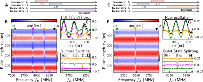
A Pulse diagram: resonant pulse of length τA driving linearized transmon A followed by pulse of frequency fB driving transmon B and readout with resonator B. B Readout resonator B response as a function of τA and fB. C Vertical line-cuts of panel B showing Rabi-like oscillation. D Horizontal line-cuts of panel B showing photon-number splitting of transmon B transition by transmon A’s excitation number \({\{\left\vert 0\right\rangle,\left\vert 1\right\rangle,\left\vert 2\right\rangle \}}_{A}\). E Pulse diagram: resonant pulse of length τB driving transmon qubit B followed by pulse of frequency fA driving linearized transmon A and readout with resonator A. F Readout resonator A response as a function of τB and fA. G Vertical line-cuts of panel F showing Rabi oscillation. H Horizontal line-cuts of panel F showing splitting of transmon A transition by transmon B’s qubit states \({\{\left\vert 0\right\rangle,\left\vert 1\right\rangle \}}_{B}\).
As a complementary experiment, we probe the system response when the nonlinear transmon B is excited first, followed by spectroscopy on linear transmon A and readout through resonator A, as described in Fig. 3E. Similar to before, we plot the phase of resonator A in Fig. 3F, and show corresponding vertical and horizontal line-cuts in Fig. 3G, H, respectively. Since transmon B has much larger self-Kerr anharmonicity of 25.44 ± 0.11 MHz (Table 1) compared to the drive amplitude, we see a Rabi oscillation expected of driven qubits in Fig. 3G. We also observe in Fig. 3H a splitting of transmon A’s transition by transmon B’s qubit states \({\{\left\vert 0\right\rangle,\left\vert 1\right\rangle \}}_{B}\), with the relative strength of each peak varying in accordance with expected qubit population oscillation during the Rabi cycle. We again extract the cross-Kerr from the \({\{\left\vert 0\right\rangle,\left\vert 1\right\rangle \}}_{B}\) splitting to be χ = 365.69 ± 0.36 MHz (see Supplementary Note 4 for details). The two cross-Kerr values show excellent agreement within measurement uncertainty and average to χ = 366.0 ± 0.5 MHz, leading to \(\tilde{\eta }=(4.852\pm 0.006)\times 1{0}^{-2}\) in the near-ultrastrong nonlinear light-matter coupling regime.
Simulated light-light nonlinear coupling
Transmon B exhibits qubit-like behavior under a weak, resonant drive in Fig. 3, but its small self-Kerr anharmonicity can be exploited under a strong, off-resonant drive to excite higher levels and exhibit resonator-like behavior instead. As shown in Fig. 4A, we repeat the experiment in Fig. 3 but now apply the first pulse with larger amplitude and a detuning of ΔA(B) = −10(+5) MHz from transmon A(B)’s f0→1 transition (see Supplementary Note 5 for detailed time domain results). This allows us to simulate the regime where both transmons are linearized or light-light nonlinear coupling. The resulting spectroscopy in Fig. 4B shows clear signature of photon-photon cross-Kerr24, with number splitting for both transmons, by \({\{\left\vert 0\right\rangle,\left\vert 1\right\rangle,\left\vert 2\right\rangle,\left\vert 3\right\rangle \}}_{A}\) and \({\{\left\vert 0\right\rangle,\left\vert 1\right\rangle,\left\vert 2\right\rangle \}}_{B}\), respectively. As expected for the same device operating point, the extracted χ is the same as in Table 1. Compared to state-of-the-art χ/2π = 2.59 MHz24, our simulated light-light coupling demonstrates more than two orders of magnitude increase in χ. We emphasize that with a greater range of flux-tunability or more precise parameter targeting in fabrication, our quartonic architecture is capable25 of demonstrating light-light nonlinear coupling with both transmons linearized to state-of-the-art levels (≤4 MHz24).
Fig. 4: Matter-matter and simulated light-light nonlinear coupling.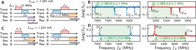
A Pulse diagrams for simulated light-light nonlinear coupling experiments at Ibias = 1.285 mA. The initial transmon A(B) drive pulse is frequency detuned from (f0→1) resonance by ΔA(B) = −10(+5) MHz to better excite higher energy level transitions. B Spectroscopies showing photon-number splitting of both transmons’ transition, a key signature of cross-Kerr between two photon modes. First 4 levels of transmon A and 3 levels of transmon B are visible with \(\{\left\vert 0\right\rangle,\left\vert 1\right\rangle \}\) splitting of χ/2π = 365.6(4) ± 0.5(3) MHz for transmon A(B). Left, right panels of number splitting results are obtained from respective left, right pulse diagrams (panel A). C Pulse diagrams for matter-matter nonlinear coupling experiments at Ibias = 1.224 mA. The initial transmon A(B) drive is a resonant π/2 pulse. D Spectroscopies showing qubit state splitting of both transmons’ transition, as expected for cross-Kerr between two qubit modes. Measured \(\{\left\vert 0\right\rangle,\left\vert 1\right\rangle \}\) splittings of χ/2π = 580.5(2) ± 0.6(4) MHz for transmon A(B). Left, right panels of qubit state splitting results are obtained from respective left, right pulse diagrams (panel C).
Matter-matter nonlinear coupling
To explore the regime of maximal nonlinear coupling with our device, we follow theory predictions of Fig. 2B and flux-bias the gradiometric quarton coupler to Ibias = 1.224 mA. This coincides with a matter-matter coupling regime where both transmons have high self-Kerr anharmonicity and thus behave as qubits or artificial atoms (see Supplementary Note 3 for detailed qubit properties). We then measure cross-Kerr coupling by performing the experiment outlined in Fig. 4C: applying first a π/2 pulse to one qubit, followed by spectroscopy of the other qubit and readout. The spectroscopy results in Fig. 4D shows the expected qubit state splitting, with an extremely large extracted cross-Kerr of χ/2π = 580.5(2) ± 0.6(4) for transmon A(B). The averaged χ/2π = 580.3 ± 0.4 MHz is, to the best of our knowledge, the largest ZZ coupling rate between two coherent qubits of any physical platform, and is equivalent to a CZ gate time of 0.86 ns. Here we exclude comparison with annealer architectures such as38 that lack measurable qubit coherence.