Dephased spin-oscillator model
The spin-boson model describes a spin coupled to a continuous bath of quantum harmonic oscillators. The Hamiltonian is given by
$$\hat{H}={\hat{H}}_{S}+{\hat{H}}_{B}+\frac{{\hat{\sigma }}_{Z}}{2}\otimes \int_{0}^{\infty }d\omega \sqrt{\frac{J(\omega )}{\pi }}\left(\hat{a}(\omega )+{\hat{a}}^{{{\dagger}} }(\omega )\right),$$
(1)
where J(ω) is the spectral density of the bath, \(\hat{a}(\omega )\) is the annihilation operator of the bath oscillator at frequency ω, and \({\hat{H}}_{S}=\frac{\epsilon }{2}{\hat{\sigma }}_{Z}+\frac{\Delta }{2}{\hat{\sigma }}_{X}\) and \({\hat{H}}_{B}=\int_{0}^{\infty }d\omega \omega {\hat{a}}^{{{\dagger}} }(\omega )\hat{a}(\omega )\) are the Hamiltonian of the spin and the bath, respectively. Here, ϵ and Δ are the detuning and coupling strength between the spin states, respectively, and ℏ is set to 1 for simplicity. We assume that the spin is initially in the \(| 0\rangle\) state (or the “donor” state in the energy transfer model) and the time evolution of the Hamiltonian induces population transfer to the \(| 1 \rangle\) state (or the “acceptor” state). Each bath oscillator of frequency ω is in the thermal state of average phonon number \(\bar{n}(\omega )=1/({e}^{\beta \omega }-1)\), where β is the inverse of the temperature (kB = 1 for simplicity).
We decompose the spectral density J(ω) of a structured bath into a sum of multiple Lorentzian peaks, each of which can be represented by a dissipative harmonic oscillator15. In this work, we consider a spin coupled to several oscillators subject to constant dephasing (“dephased” spin-oscillator model). This discrete oscillator model is described by the Hamiltonian
$${\hat{H}}_{D}={\hat{H}}_{S}+{\sum}_{l}\frac{{\kappa }_{l}}{2}{\hat{\sigma }}_{Z}\otimes ({\hat{b}}_{l}+{\hat{b}}_{l}^{{{\dagger}} })+{\sum}_{l}{\nu }_{l}{\hat{b}}_{l}^{{{\dagger}} }{\hat{b}}_{l}$$
(2)
and corresponding Lindblad operators \({\hat{L}}_{l}={\sqrt{\Gamma }}_{l}{\hat{b}}_{l}^{{{\dagger}} }{\hat{b}}_{l}\), where κl represents the coupling strength between the spin and l-th oscillator, νl and Γl denote the frequency and the dephasing rate of the l-th oscillator, respectively, and \({\hat{b}}_{l}\) is the annihilation operator of the l-th oscillator. The composite state ρ of spin and oscillators follows the Lindblad master equation \(\dot{\rho }=-i[{\hat{H}}_{D},\rho ]+{\sum }_{l}({\hat{L}}_{l}\rho {\hat{L}}_{l}^{{{\dagger}} }-\frac{1}{2}\{{\hat{L}}_{l}^{{{\dagger}} }{\hat{L}}_{l},\rho \})\). In a reasonable regime of parameters (Γl νl /2, \(\beta \ll 2\pi {({\Gamma }_{l}/2)}^{-1}\))15, this bath of dephased oscillators is assigned a spectral density composed of Lorentzian peaks
$${J}_{{{{\rm{Lo}}}}}(\omega )={\sum}_{l}{\kappa }_{l}^{2}\left(\frac{{\Gamma }_{l}/2}{{({\Gamma }_{l}/2)}^{2}+{(\omega -{\nu }_{l})}^{2}}-\frac{{\Gamma }_{l}/2}{{({\Gamma }_{l}/2)}^{2}+{(\omega+{\nu }_{l})}^{2}}\right),$$
(3)
where we assume that each oscillator is initially in the thermal state with average phonon number \(\bar{n}({\nu }_{l})\).
The spectral density of the bath determines the dynamics of the spin to leading order in \(\bar{\kappa }T\), where \(\bar{\kappa }\) is the average coupling strength and T is the evolution time (see Section III of the Supplementary Material). Therefore, the spin dynamics of the dephased spin-oscillator model approximately match those of the spin-boson model with J(ω) = JLo(ω) in the weak-\(\bar{\kappa }\) regime. In the unbiased (ϵ = 0) spin-boson model1,29,30,31, the equilibrium donor-state population is 1/2 for both models, and we expect the population dynamics of the two models show an excellent match at all times for weak spin-bath coupling (Supplementary Fig. 4). For the case of biased spin-boson models in the stronger coupling regime (ϵ ≠ 0, such as discussed in the VAET case), the dynamics of the dephased spin-oscillator model we simulate can deviate significantly from the traditional spin-boson model.
A more common model for dissipation is a spin coupled to oscillators subject to constant damping (“damped” spin-oscillator model) described by a pair of Lindblad operators \({\hat{L}}_{l1}=\sqrt{{\Gamma }_{l}(\bar{n}({\nu }_{l})+1)}{\hat{b}}_{l}\) and \({\hat{L}}_{l2}=\sqrt{{\Gamma }_{l}\bar{n}({\nu }_{l})}{\hat{b}}_{l}^{{{\dagger}} }\)15,16, where Γl here is the damping rate of the l-th oscillator. A stronger result holds for this model: the spin dynamics are non-perturbatively equivalent to those of the spin-boson model with the same spectral density, up to all orders in \(\bar{\kappa }T\)32. Damped oscillators can be realized in trapped ions using sympathetic cooling on a chain of ions with multiple atomic species or isotopes15,16, or using qubits encoded in different internal-state manifolds of the same type of ions33. In fact, a recent work reported simulation of electron-transfer model using sympathetic cooling on the motional mode of a trapped ion34. The dephased oscillator model developed in this work expands the ability to simulate a broader set of bath models not experimentally accessible before.
Experimental implementation
The simulations of spin-boson models are performed using a linear chain of seven 171Yb+ ions (Fig. 1). Two hyperfine internal states (\(| 0 \rangle\) and \(| 1 \rangle\)) are used to represent the spin (or qubit). The ions sit 68 μm above the surface of the trap35, and the heating rate and decoherence time of the zig-zag motional mode are 3.6(3) quanta/s and 5.2(7) ms, respectively. The other motional modes used have similar magnitudes. Details of our experimental setup can be found in Ref. 36. Using Doppler, electromagnetically-induced transparency (EIT), and sideband cooling techniques, the zig-zag motional mode can be cooled to near ground state with \(\bar{n}=0.036(16)\). Standard qubit manipulation techniques can be used to initialize and measure the qubits, and single-qubit operations are driven by stimulated Raman transitions. The spin-oscillator coupling is simulated using the spin-dependent kick (SDK) operation induced by simultaneous application of blue- and red-sideband transitions (see Methods).
Fig. 1: Schematic of the experimental setup.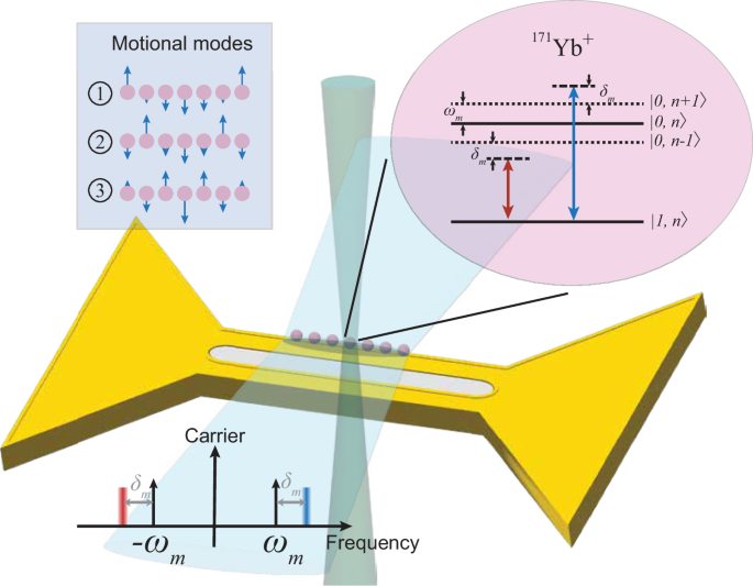
The ions are confined in a micro-fabricated surface trap. The spin states are encoded as the hyperfine clock states (qubit states) and the bosonic bath modes are encoded as the collective radial motional modes of the ion chain. We strategically use the center ion and the three symmetric modes (except for the center-of-mass mode, as shown in the upper left corner) in the experiment to minimize cross-mode couplings (see Methods). The laser frequencies for the SDK operations are determined by the frequency difference between the two Raman beams, and are depicted by the red and blue lines on the frequency axis detuned by δm from the mode frequency ωm, with the color gradients indicating the random frequencies used to implement the decoherence simulation.
The evolution of \({\hat{H}}_{D}\) in Eq. (2) is mapped to a sequence of single-qubit rotations and SDK operations via Trotterization. We apply time evolution operators over a short time interval corresponding to each term in the Hamiltonian in the interaction picture, and repeat them over many time intervals to simulate the evolution dynamics (see Methods). This approach can be readily extended to simulating more complicated molecular models consisting of many electronic states and bath modes18,37.
The dephased spin-oscillator model can be simulated using trapped ions by applying the SDK operations, which induce the coupling between the qubit and the motional mode. By adding randomness to the control parameters of the SDK operations and averaging the results over many random trials, we can implement dissipative processes such as preparing the thermal state and simulating the dephasing of the motional mode. The key idea is that certain dissipative evolutions described by the Lindblad master equation are equivalent to an average of many coherent evolutions, each subject to a stochastic Hamiltonian38. Details of the procedure is described in Methods.
Single-oscillator case
We first consider a single-oscillator case (l = 1), and demonstrate the programmability of the bath’s initial temperature quantified by the oscillator’s average phonon number \(\bar{n}\). Controlled amounts of resonant SDK operations with stochastically varying phase are applied to the ion prepared near the motional ground state, which prepares the thermal state equivalent to an ensemble of randomly displaced coherent states (see Methods). Figure 2a illustrates the simulated time evolution of the donor state population when it is coupled to such initial bath state, for various values of \(\bar{n}\). The dynamics exhibit coherent oscillations with an envelope of slow collapse and revival (beat-note) that signifies resonant (ν1 = Δ) energy exchange between the system and the bath oscillator39. A thermal state of larger \(\bar{n}\) is a mixture of wider range of coherent states, leading to reduced beat-note amplitude at t ≈ 2π/Δ × 10.5.
Fig. 2: Demonstration of the tunability of the bath’s initial temperature and spectral linewidth.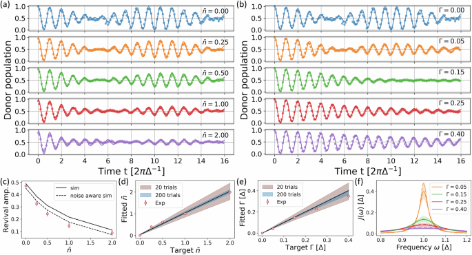
a Dynamics of the coherent spin-single oscillator model \({\hat{H}}_{D}\) with various values of average phonon number \(\bar{n}\) for the oscillator’s initial state. b Dynamics of the model with \(\bar{n}=0\), J(ω) = JLo(ω) (single peak) and various values of Γ1 ≡ Γ. For both (a) and (b), ϵ = 0, ν1 = Δ, and κ1 = 0.1Δ. Lines and dots represent theoretical predictions and experimental data, respectively. The error bars (size comparable to the symbols in these two plots) denote measured standard deviation over 20 trials, each trial performed with randomly drawn set of parameters and repeated 100 times. c Revival amplitude versus \(\bar{n}\). Predictions of the original (solid line) model and the noise-aware (dashed line) model are compared with the experimental results (circles). d Measured values of \(\bar{n}\) fitted to the predictions of the noise-aware model. The solid line depicts \(y=x+{\bar{n}}_{0}\), where \({\bar{n}}_{0}=0.036\) is the expected offset in the phonon number due to imperfect cooling. e Measured values of Γ fitted to the theoretical predictions with \(\bar{n}={\bar{n}}_{0}\). The solid line depicts y = x. In (d) and (e), the blue and brown shaded regions represent the expected uncertainty of the value when the populations are averaged over 20 and 200 random trials, respectively. f Lorentzian spectral densities for various target (solid) and fitted (dashed) values of Γ. The shaded region represents the expected uncertainty of Γ when averaged over 20 random trials.
We compare our experimental results with the predictions of “noise-aware” models, reflecting inherent noise processes in the experimental setup. We fit the experimental data using an oscillator model with initial phonon number \(\bar{n}+{\bar{n}}_{0}\) and Lorentzian spectral density with full width at half maximum (FWHM) Γ1 ≡ Γ [Eq. (3)], where the values \({\bar{n}}_{0}=0.036\) and Γ = 0.0022Δ are extracted from independent measurements characterizing imperfect cooling and finite motional coherence time, respectively. The experimentally measured revival amplitude (Fig. 2c) and fitted \(\bar{n}\) (Fig. 2d) match well with the predictions of noise-aware models. This shows that well-characterized experimental noise can serve as the baseline values for the thermal excitation and dephasing rate in the open quantum system model, and thus is not always a bottleneck for the accuracy of our simulations.
Next, we show the tunability of the dephasing rate Γ, which corresponds to the linewidth of the spin-boson model’s spectral density. Dephasing is implemented by adding random frequency offsets to the SDK operations that simulate the time evolution (see Methods). This mimics the random fluctuations of the motional-mode frequency, following the stochastic model of motional dephasing noise in trapped-ion systems36.
Figure 2 b illustrates the dynamics for various values of Γ between 0 and 0.4Δ, which exhibit a crossover from underdamped to overdamped dynamics as Γ is increased (critical damping condition at Γ ≈ 0.18Δ). As the damping is increased beyond the critical point, the beat-note that signifies the excitation transfer from the spin to boson back to spin is suppressed, and there is a monotonic decrease in the oscillation of the donor population in the overdamped regime. We notice a π phase flip in the oscillation of the donor population in the beat-note in the underdamped case, signified by the phase difference between the underdamped and overdamped cases at t ≈ 2π/Δ × 10.
The uncertainty of \(\bar{n}\) and Γ realized in the experiment can be reduced by performing a larger number of random trials, each trial using a different set of random parameters. The shaded areas in Fig. 2d and e show the standard deviation of fitted values for \(\bar{n}\) and Γ, obtained by numerical simulation of results averaged over 20 (pink) or 200 (blue) random trials. Our experiments are limited to 20 random trials due to the compiling delay required for each set of control parameters, and each trial is repeated 100 times to obtain the expectation value for the donor population. The experimental data is consistent with the standard deviation derived from 20 numerical trials. We expect to readily increase the number of random trials with fewer repetitions each in future experiments with faster compilation tools40.
Engineering bath spectral densities
We can use multiple oscillator modes to engineer a target spectral density structure for the oscillator bath. We simulate a bath of spectral density composed of up to 3 Lorentzian peaks, each represented by a motional mode of the ion chain. The bath spectral density J(ω) in Fig. 3a is simulated using the SDK operations over two or three motional modes. Figure 3b shows the frequencies of the laser pulses used to drive the SDK, defined as the detuning of laser beams from the carrier transition frequency. The 1st, 3rd, and 5th motional modes are used, and the detuning of the laser frequency from each motional mode determines the frequency at which the bath spectral density is considered in Fig. 3a. We set the electronic coupling strength Δ = 500 cm−141, such that at temperature 77 K, \(\bar{n}\approx 0.1\) for the near-resonance vibrational modes. Figure 3c shows the results for simulating the dynamics of spin-boson models with spectral densities composed of 2 and 3 Lorentzian peaks, respectively. The theoretical predictions are obtained using the time-dependent density-matrix renormalization group algorithm in the interaction picture42. The donor population features underdamped coherent oscillations, with contributions from all three modes. The measured population closely follows the theoretical predictions.
Fig. 3: Simulations of molecular energy transfer in model structured baths.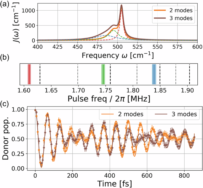
a Simulated spectral density of the spin-boson model’s bath, where the electronic coupling strength Δ = 500cm−1. The orange and brown solid curves illustrate the spectral densities summed over two and three peaks, respectively. b Dashed lines represent the radial motional modes that are coupled by the Raman beam. Black or grey dashed lines represent modes with non-zero or zero coupling strength to the target ion, respectively. The three solid lines and the shaded regions depict the mean value and the standard deviation of the randomized pulse frequencies, and the color corresponds to the Lorentzian peak generating the final spectral density in (a). c Time evolution of the spin-boson models with J(ω) in (a). The x-axis represents the simulated time of the chemical model, determined by the chosen model parameters (see Section I of the Supplementary Material). The bath temperature is 77 K such that \(\bar{n}\approx 0.1\), which is set for trapped ions’ motional modes using imperfect sideband cooling. Curves and dots represent theoretical predictions and experimental data, respectively. Error bars are derived as in Fig. 2.
The coherence time of the motional modes in our setup of ~5.2(7) ms is the leading source of noise36,43, and is comparable to the experimental time for simulating the time evolution under spectral densities generated from 2 mode (1.63 ms) and 3-mode (2.56 ms) cases. For these simulations, the contribution of motional decoherence in the experiment is identical to the random kicks that we apply in the spin-oscillator model to simulate the bath, and can be incorporated as the source of dephasing in our simulation with proper calibration43.
Leggett spin-boson models
We further simulate the spin-boson models inspired by Leggett et al.1. The spectral density of the bath is given by
$${J}_{{{{\rm{Legg}}}}}(\omega )=A{\omega }^{s}{\omega }_{c}^{1-s}{e}^{-\omega /{\omega }_{c}},$$
(4)
where ωc is the cutoff frequency, and s s = 1, and s > 1 represent the sub-Ohmic, Ohmic, and super-Ohmic baths, respectively. This model is widely used to characterize the noise in nanomechanical devices44, superconducting circuits12,45, and proton-transfer reactions46,47. The spin dynamics exhibit various behaviors, such as coherent oscillations, incoherent decay, and localization, depending on the values of s and A, which has been a subject of longstanding research using analytical tools1,48 and classical simulations29,30,31,49.
Recognizing that the spin exchanges energy with the bath only near its resonance, we use a sum of Lorentzian lines from motional modes to approximate the spectral density JLegg(ω) near the resonance frequency Δ, with the cutoff frequency set to be much higher (ωc = 10Δ). We utilize well-established global optimization algorithms to find the optimal set of parameters (κl, Γl, and νl in Eq. (3)) that best represent JLegg(ω) (see Section V of the Supplementary Material). Using this approach, we consider weak spin-bath coupling (A = 0.1) and match the spectral density within the target bandwidth ω ∈ [0.9Δ, 1.1Δ] with 2 Lorentzian peaks. Figure 4a shows the obtained spectra from the modes (solid lines) that approximate the spectral densities (dot-dashed lines) with s = 0.5, 1.0, and 2.0, respectively. The results for the donor population dynamics interacting with a bath featuring these approximated spectral densities are shown in Fig. 4b–d. We observe a crossover from near-coherent (s = 2) to fully damped (s = 0.5) oscillations in the simulated time scale, owing to the different levels of spectral density J(ω = Δ) near resonance. The experimental data match well with theoretical predictions, where the deviations in Fig. 4d result from an insufficient number of Trotterization steps (Supplementary Fig. 5). Simulations of baths with fixed J(ω = Δ) value over varying levels of the s parameter (ranging from s = 0.3 to s = 3) are shown in Section VI of the Supplementary Material (Supplementary Fig. 6).
Fig. 4: Simulations based on Leggett’s spin-boson model.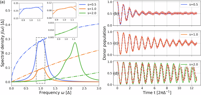
a Spectral densities of the Leggett’s model. Dot-dashed curves are the sub-Ohmic (s = 0.5), Ohmic (s = 1.0), and super-Ohmic (s = 2.0) spectral densities described by Eq. (4) (A = 0.1, ωc = 10Δ). Solid curves are the spectral densities simulated in our experiments using two motional modes. These spectral densities are designed to match the dot-dashed curves near ω = Δ. Insets compare the solid and dot-dashed curves within the interval ω ∈ [0.85Δ, 1.15Δ]. (b)(c)(d) Dynamics of the spin-boson model for s = 0.5, 1.0, and 2.0, respectively. The solid curves represent the theoretical predictions of the spin-boson models with spectral densities given by the solid curves in (a). The red dashed curves are expected results, derived from numerical simulations of the density matrix of the qubit and motional modes subject to control operations and hardware noise. Circles denote experimental data and error bars indicate the standard deviation over 60, 20, and 20 trials for (b), (c), and (d), respectively (More trials were needed to overcome the shot noise in (b) when the donor population is near 0.5).
Vibration-assisted energy transfer
Finally, we simulate the VAET model24 with nonzero energy detuning ϵ between the spin states. Here we set the spin parameters as Δ = 30cm−1 and ϵ = 100cm−1. In the absence of coupling to a vibrational mode (κ = 0cm−1), energy transfer between the detuned spin states is suppressed; however, for nonzero κ, the energy transfer can be activated if the mode frequency ν meets the resonance condition (single mode’s index l = 1 omitted).
Figure 5a shows the experimental data for simulating the coherent spin-single oscillator model \({\hat{H}}_{D}\) with a relatively large coupling strength (κ = 30cm−1). When ν satisfies the resonance condition of VAET (\(\nu=\sqrt{{\Delta }^{2}+{\epsilon }^{2}}/k\approx 104 {{\mbox{cm}}}^{-1}/k\) where k is an integer), energy transfer occurs24. Otherwise, energy remains localized at the donor state. Figure 5b shows the impact of initial temperature of the oscillator on the resonant VAET (ν = 104cm−1). We create baths of two temperatures 0 K and 300 K corresponding to initial average phonon number \(\bar{n}=0\) and 2.0, respectively. The energy transfer is faster for higher \(\bar{n}\) in the beginning as more vibrational quanta assist the energy transfer, but it also leads to a rapid decay of oscillations over time as the coherence is lost.
Fig. 5: Simulations of vibration-assisted energy transfer (VAET).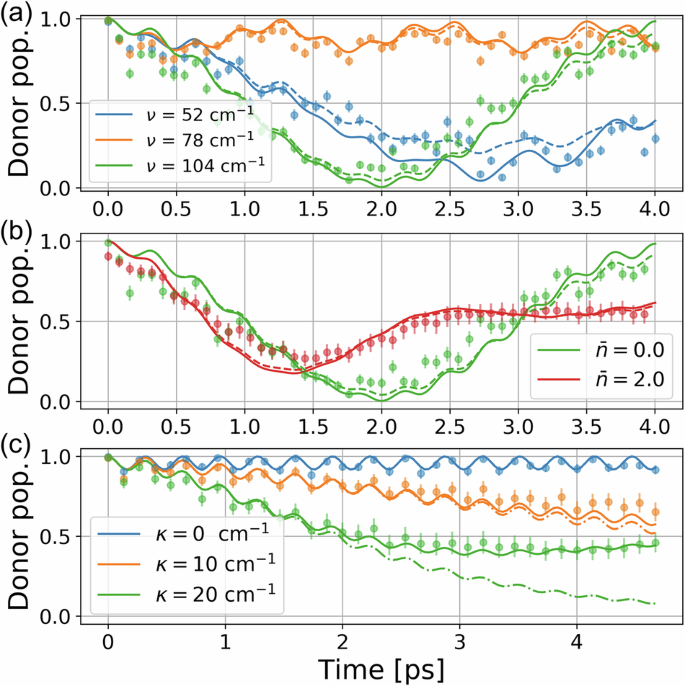
We set ϵ = 100 cm−1 and Δ = 30 cm−1. The x-axis represents the simulated time of the chemical model, determined by the chosen model parameters (see Section I of the Supplementary Material). a, b Time evolution of the donor-state population for coherent VAET models with κ = 30 cm−1. Solid and dashed curves depict theoretical predictions of the ideal target and the noise-aware model, respectively. Circles represent experimental data and error bars are the standard deviation over 100 repetitions. In (a), bath temperature is fixed at 0 K (\(\bar{n}=0\)) and ν is varied. In (b), ν is fixed to the resonant value 104 cm−1 and two temperatures 0 K and 300 K, which correspond to \(\bar{n}=0\) and 2.0, respectively, are simulated. c Time evolution of the donor-state population for dissipative VAET models with ν = 104 cm−1 and Γ = 10cm−1 at 0 K. Solid and dot-dashed curves depict theoretical predictions of the dephased spin-oscillator model and the damped spin-oscillator model, respectively. Circles denote experimental data. For κ = 0cm−1, error bars indicate the standard deviation over 100 repetitions. For κ = 10 and 20 cm−1, error bars indicate the standard deviation over 20 trials, each trial performed with a randomly drawn set of parameters and repeated 100 times.
In Fig. 5c, we simulate the dephased spin-oscillator model with Γ = 10cm−1 and various values of κ, to study the impact of dissipative coupling. We note that in the weak-κ regime (or short evolution time), the results agree with the theoretical predictions of the damped spin-oscillator model, which is equivalent to those of the spin-boson model with J(ω) = JLo(ω)15,32; however, as κ is increased, the dephased and damped models’ dynamics deviate. This is expected because, unlike the damped model, the dephased model does not extract energy from the spin-oscillator system, so the donor population will not decay towards zero even after a long time evolution when coupled to a single-oscillator bath. This example demonstrates that our method provides the ability to simulate a wider range of dissipative channels in the study of open system dynamics.