Here, we detail the methodology employed to generate the high-resolution pesticide maps. Our work takes 2018 as the reference year, selected based on the availability of crops spatial mapping data. Figure 1 illustrates the workflow of the implemented methodology while all steps are detailed below.
Fig. 1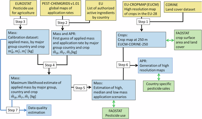
Schematic diagram of the proposed procedure. Yellow boxes indicate input data, blue boxes data analysis steps and green boxes validation data employed. Black and blue lines identify the procedure leading to the estimation of application rate maps (APR) and data quality maps, respectively.
Step 1. European crop maps selection and aggregation
The crop maps are required to apply the original PEST-CHEMGRIDSv1.01 framework17 and generate high-resolution pesticides application rates maps in EU. The goal of this step is to (re)construct from available sources a spatial dataset featuring the 10 cropping systems in PEST-CHEMGRIDv1.01, i.e. Corn, Soybean, Wheat, Cotton, Rice, Alfalfa, Vegetable and Fruits, Orchard and grapes, Pasture and Hay, and Other crops.
The high-resolution EU crop map (EUCM, d’Andrimont et al.20) is the key source of information, as it provides crops spatial distribution at 10 m resolution over the whole EU-28 area. The dataset is obtained combining satellite and in situ observations of cropping systems through the LUCAS survey. We then manipulated EUCM with two objectives: i) integrating EUCM with the CORINE land cover21 dataset to resolve some specific limitations in EUCM that are also acknowledged by the authors20, ii) elaborate labels to optimize matching with crop categories that are present in PEST-CHEMGRIDSv1.01. From an operational standpoint, data embedded in EUCM are corrected in the following cases:
-
Rice pixels are retrieved from CORINE; thus when a pixel is labelled as “rice” on CORINE, we replace the EUCM value with “rice”.
-
While the EUCM label “Woodland and Shrubland (including permanent crops)” contains important information for identifying woody permanent crops, it does not discern other type of vegetation covers. Hence, we selected pixels that are assigned such categories in EUCM and are categorized as “vineyards”, “fruits trees and berry plantations” or “olive groves” on the CORINE land cover dataset. These pixels are classified as “Orchards and Grapes”, consistent with PEST-CHEMGRIDSv1.01.
-
All “Grasslands” grid-cells in EUCM that appeared as “Pastures” in CORINE, were eventually considered as “Pastures” in EUCM.
After integration of the two datasets, map resolutions were changed to 250 m, assigning to each pixel in the upscaled map the modal value of the pixels (of 10 m resolution) included in the original map. The upscaling procedure is motivated by our goal of mapping a large number of pesticides application rates. Maintaining a 10 m resolution would complicate data handling without significantly increasing the dataset spatial significance. This map is labeled here as EUCM-CORINE-250.
Map labels are then arranged to match the PEST-CHEMGRIDSv1.01 crop categories as reported in Table 1. The taxonomy of aggregated crop classes resulting from the EUCM-CORINE-250 map is shown in Supplementary Information (Table S2), where entries are gathered from LUCAS and CORINE documentation. The following considerations can be made:
-
Crop matching is unambiguous across all datasets for classes Maize, Wheat, Soya and Rice.
-
Alfalfa falls into the category Fodder crops in EUCM. We have found no sources to distinguish alfalfa from other fodder crops (cereals and other leguminous). Similarly, Cotton is included in “other industrial crops” in EUCM along with other crop types. Therefore we exclude alfalfa and cotton from the analysis.
-
Aggregated classes Vegetable and Fruits and Orchard and Grapes defined by USGS, and used in PEST-CHEMGRIDSv1.01 (see Table 2) are reasonably met in EUCM-CORINE-250.
Table 1 Correspondence between EUCM-CORINE-250 and PEST-CHEMGRIDS (PCG in the table) crop classes and percentage of surface area (SA) associated with each label.
Table 2 Taxonomy of considered active ingredients, major groups and chemical class definitions (CClass) and names are taken from EUROSTAT.
Because of the exclusion of two crop types Cotton and Alfalfa, our maps consider eight of the ten classes included in PEST-CHEMGRIDSv1.01 (see Table 1). The EUCM-CORINE-250 map is georeferenced using the EPSG:3035 projected coordinates.
Step 2. Projection of PEST-CHEMGRIDSv1.01 maps onto fine grid and screening of active ingredients
We perform a projection of PEST-CHEMGRIDSv1.01 maps onto the same georeferenced grid used to map crops in Step 1. For each pixel in EUCM-CORINE-250 we interpolate crop-specific value of application rates provided by PEST-CHEMGRIDSv1.01 using a nearest neighbour approximation. While performing this operation, we apply country-specific pesticides use authorizations and bans for active ingredients as of January 9th 2018. Overall, we obtain a list of 55 active ingredients approved in at least one country. These are categorized following the EUROSTAT22 nomenclature, i.e., into ‘major groups’ (e.g., ‘herbicides’, label H) and ‘chemical class’ (e.g., ‘phenoxy herbicides’, label H01_01). Each chemical class contains a variable number of active ingredients (ais). The considered active ingredients pertain to 37 distinct chemical classes and four major groups, as reported in Table 2. Note that in our dataset there are only two active ingredients belonging to the major group “other plant protection product”, hence the active ingredients Metam and Metam potassium are disregarded in this work. In the following, we thus focus on major groups herbicides, haulm destructors and moss killers (H), fungicides and bactericides (F) and insecticides and acaricides (I). These groups are referred to as herbicides, fungicides and insecticides for brevity. All chemical classes and the matching active ingredients included in our dataset are reported for completeness in Table 2, along with the indication of the crop to which they apply in our analysis, this information being retrieved from the PEST-CHEMGRIDv1.01 framework. After projecting the maps onto the refined grid, we obtain spatial values of \({\mathop{APR}\limits^{ \sim }}_{ai}(x,y)\) [kg/ha] which define the application rate of each active ingredient ai as well as the total applied mass for each major group per crop and country, \({\widetilde{m}}_{{mg}}({crop},{country})\) [kg], with mg = H, F, I.
Step 3. Preprocessing of calibration data
Here, we assemble a calibration dataset to update the preliminary estimates obtained using PEST-CHEMGRIDv1.01. We collect a calibration dataset from EUROSTAT22, which is hereafter denoted as reference dataset. The following steps are performed to obtain a calibration dataset from the reference dataset:
-
a.
Data included in the reference dataset are sparse in time; therefore, we consider average quantities from 2015–2020 to obtain reference data to 2018.
-
b.
We select applied mass related to chemical classes containing one or more active ingredients included in the PEST-CHEMGRIDSv1.01 dataset, as shown in Table 2.
-
c.
The reference dataset indicates crop type, mass, and chemical class of active ingredients. We subdivide data between three different crop classes. We categorize as “Wheat” the applied mass associated with crop labels “Common spring wheat and spelt”, “Common wheat and spelt “, “Common winter wheat and spelt”, “Durum wheat”. We classify as “Corn” the applied mass associated with crops labelled as “Grain maize and corn-cob-mix” and “Green maize”. Composite crop classes are grouped together to avoid possible misclassification due to nonmatching labels. Note that we could exclude data related to “Soybeans” and “Rice”, which represent a very limited portion of crop area in our study. Therefore, these are grouped with other composite crop classes in a “Any Other Crop” (AOC) class.
-
d.
We neglect applied mass per country and crop class whose value is smaller than 100 kg.
Upon performing the above steps, we obtain a set of 175 applied mass data, each representing a pesticide mass applied per country, crop and pesticide major group (herbicides, fungicides and insecticides, here labelled as F, H, I). The whole dataset is then split according to the three major groups. We label these data as \({F}_{mg}^{\ast }={m}_{mg}^{\ast }({crop}{,}{country})\) [kg] where mg stands for F, H, I, crop = [“Corn”, “Wheat”, “AOC”] and country indicates the EU-28 Countries (see Supplementary information, Table S1).
The selection performed in steps a.-f., described above, implies that our reference dataset includes a subset of the available data reported in EUROSTAT. We quantify here the significance of the considered data over the total figures reported in EUROSTAT for the three considered major groups. Figure 2 displays the ratio \({F}_{mg}^{\ast }={m}_{mg}^{\ast }({crop}{,}{country})/{m}_{mg}^{\ast }({crop}{,}{country})\), where \({m}_{mg}^{\ast }\)(crop,country) represents the cumulative mass associated with each of the three major groups considered, thus including all chemical classes pertaining to a major group. Note that when \({F}_{mg}^{\ast } > 1\), the value is disregarded. This can happen due to asynchronous reporting of major groups and underlying chemical classes in EUROSTAT. We observe that the major group best represented in our data product is herbicides, followed by fungicides and insecticides. The selected applied mass data \({m}_{mg}^{\ast }\) represent 83.6%, 42.4% and 27.4% of the total herbicide, fungicide and insecticide mass reported in EUROSTAT, respectively. These fractions are labeled as \({\overline{F}}_{H}^{\ast },{\overline{F}}_{F}^{\ast },{\overline{F}}_{I}^{\ast }\) in the following. Considering the mass applied per crop, our dataset includes 82.3%, 81.0% and 48.3% of the total pesticide mass applied for Corn, Wheat and Any Other Crop classes, respectively. We also note that the available data are mostly complete for Wheat, while missing data are relatively more abundant for Corn. The total mass included in our dataset collectively represents 55.4% of the total mass that can be obtained considering the cumulative applied mass of H, F, and I reported in EUROSTAT.
Fig. 2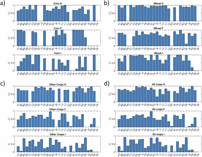
Mass fraction of active ingredients retained in our reference dataset as compared to total mass by major group reported in EUROSTAT for Herbicides (H), Fungicides (F) and Insecticides (I). Results are for (a) Corn, (b) Wheat, (c) Any Other Crop, (d) mass-weighted average for all crops.
Step 4. Calibration of applied pesticide mass
Adjustment of the applied pesticides mass by major group is performed assuming the following scaling model based on geographical location and crop type
$${m}_{{mg}}={k}_{{mg},C}{\left({crop}\right)k}_{{mg},L}\left({country}\right){\widetilde{m}}_{{mg},{PCG}}{\left({country},{crop}\right)}^{\alpha }$$
(1)
where \({\widetilde{m}}_{{mg}}\) is the ‘first guess’ applied mass obtained in step 2. Parameters appearing in (1) are defined as follows
$${k}_{{mg},C}\left({crop}\right)=\left\{\begin{array}{ll}{k}_{{mg},{Corn}} & {if\; crop}={corn}\\ {k}_{{mg},{Wheat}} & {if\; crop}={wheat}\\ {k}_{{mg},{AOC}} & {if\; crop}={AOC}\end{array}\right.$$
(2)
$${k}_{{mg},L}\left({country}\right)=\left\{\begin{array}{cc}{k}_{{mg},{SEU}} & {if\; country}\in {SEU}\\ {k}_{{mg},{CEU}} & {if\; country}\in {CEU}\\ {k}_{{mg},{NEU}} & {if\; country}\in {NEU}\end{array}\right.$$
(3)
with
-
SEU = [Bulgaria, Greece, Spain, France, Italy, Cyprus, Malta, Portugal]
-
CEU = [Belgium, Czech Republic, Germany, Ireland, Luxembourg, Hungary, Netherlands, Austria, Poland, Romania, Slovenia, Slovakia, United Kingdom]
-
NEU = [Denmark, Estonia, Latvia, Lithuania, Finland, Sweden]
corresponding to the southern (SEU), central (CEU) and northern (NEU) Europe countries as defined by the relevant EU directive23. For each major group, the parameters vector is thus defined as kmg = [kmg, Corn,kmg,Wheat, kmg,AOC, kmg,SEU, kmg,CEU, kmg,NEU, α]. Parameters are estimated within a maximum likelihood (ML) framework by minimizing the following objective function
$$J=\mathop{\sum }\limits_{i=1}^{3}\mathop{\sum }\limits_{j=1}^{28}{({\log }_{10}{m}_{{mg}}^{\ast }({cro}{p}_{i},{countr}{y}_{j})-{\log }_{10}{m}_{{mg}}({cro}{p}_{i},{countr}{y}_{j}))}^{2}$$
(4)
Log-transformed values are employed because of the large disparity between applied mass across the dataset. Best estimate of \({{\bf{k}}}_{{mg}}\), \({\hat{{\bf{k}}}}_{{mg}}\), is retrieved by minimizing J through the Matlab function fmincon. All parameter values are initialized equal to 1, thus assuming \({\widetilde{m}}_{{mg}}\) as a first guess solution. The ML best estimate of mmg is labelled as \({\hat{m}}_{{mg}}\). Along with parameters best estimates we obtain the minimum value of the negative log-likelihood (NLL), as well as an estimate of the posterior parameter covariance matrix24, from which we retrieve the value of the posterior standard deviation, σ, for each parameter estimate.
Calibration results are shown in Fig. 3 and Table 3. The most accurate results are obtained for herbicides, as confirmed by NLL values (lower NLL indicates higher fidelity in reproducing data). This result is consistent with the observation that our dataset provides a relatively high coverage over this class in each country and crop type. Parameter estimation uncertainty is limited for all three major groups, as inferred from the low values of σ.
Fig. 3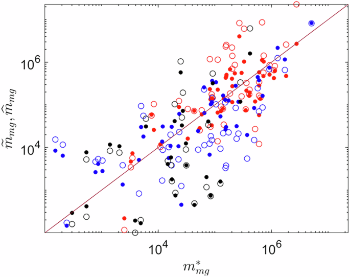
Scatter plot showing the comparison between \({m}_{{mg}}^{\ast }\) (horizontal axis), and \({\widetilde{m}}_{{mg}}\) (empty symbols), \({\hat{m}}_{{mg}}\) (filled symbols) (vertical axis). Results are for \({mg}=H\) (red symbols), \({mg}=F\) (blue symbols), \({mg}=I\) (black symbols), the continuous line indicates the axes bisector.
Table 3 Calibration results.Step 5. Estimation of uncertainty in the mass of applied pesticides
We generate Monte Carlo realizations of the total mass of applied pesticides. These are obtained upon propagating uncertainty in the parameter estimates to the estimated mass of pesticides. For each major group, we consider the estimated parameters to be independent and normally distributed with mean equal to \({\hat{{\bf{k}}}}_{{mg}}\) and standard deviations as listed in Table 3. The assumption of independence neglects potential correlations between parameters. This is considered as a cautionary measure, as correlation effects may constrain the sampling space limiting sampling to specific portions of the parameter space. The assumption of normality is commonly employed in uncertainty quantification studies when detailed prior information on the statistical distributions of parameters is lacking. We then generate a Monte Carlo sample of 103 realizations of mmg (crop,country) using Eq. (1). From this sample, we denote the first and third quartiles as the low and high estimate of pesticide applied mass, respectively. The median value is also retained, as the nonlinear Eq. (1) may lead to skewed mass distributions. We verified that the sample size yields appropriate estimates of uncertainty bounds, where variations of the related high, low, and median estimate as a function of the number of realizations is below 5%.
Step 6. Generation of pesticide maps
We calculate the following correcting factors
$$\begin{array}{ccc}{K}_{mg,S}=\frac{{m}_{mg,S}}{{\tilde{m}}_{mg}} & with & S=High,Median,Low;mg=H,F,I\end{array}$$
(5)
where \({m}_{{mg},S}\) [kg] denotes the applied mass associated with scenario S (i.e., high, median, and low estimate of pesticide applied mass). The spatially distributed application rates for all active ingredients are computed applying the correction factors
$$\begin{array}{ccc}AP{R}_{ai,S}(x,y)={K}_{mg,S}{\tilde{APR}}_{ai}(x,y) & with & High,Median,Low\end{array}$$
(6)
Because each grid cell has a fixed surface area of 6.25 ha in the used projection, the proportionality indices \({K}_{{mg},S}\) obtained from the estimate of applied mass can be directly used to determine the application rates, maintaining the cumulative mass values which is the data employed in the estimation process. Maps are discretized by considering a constant value of \({{APR}}_{{ai},S}\) for each grid cell of the map. All maps are georeferenced in the EPSG:3035 reference system.
Step 7. Data accuracy assessment
Data accuracy estimation is provided according to the estimation residuals obtained for each active ingredient major group and country, when compared with the calibration dataset (see step 3)17
$${QI}=1-\frac{|{\hat{m}}_{{mg}}({crop},{country})-{m}_{{mg}}^{\ast }({crop},{country})|}{{\hat{m}}_{{mg}}({crop},{country})+{m}_{{mg}}^{\ast }({crop},{country})}\forall {ai}\in {mg},{mg}=H,F,I$$
(7)
The value of QI is provided as spatial map using the same grid used to map application rates. When data for a given (crop,country) pair is not available we average the indicators obtained for the same country group (NEU, CEU, SEU) for the same crop.