Exact Boltzmann transport approach
To quantify the current-induced spin accumulation in tellurium crystals, we use the semiclassical Boltzmann equation25. It describes the time evolution of the electron distribution function, fk, under external stimuli:
$$\frac{\partial {f}_{{{\boldsymbol{k}}}}(t)}{\partial t}+(-e){{\boldsymbol{E}}}\cdot \frac{\partial {f}_{{{\boldsymbol{k}}}}(t)}{\hslash \,\partial {{\boldsymbol{k}}}}={\left(\frac{\partial {f}_{{{\boldsymbol{k}}}}}{\partial t}\right)}_{{{\rm{col}}}},$$
(2)
where k is the reciprocal vector, E is the applied electric field, and (−e) 2) accounts for scattering processes with impurities. While the Boltzmann equation allows us to compute charge and spin transport properties, it is challenging to solve without approximations.
A common approach to solving this equation is the relaxation time approximation25, given by \({(\frac{\partial {f}_{{{\boldsymbol{k}}}}}{\partial t})}_{{{\rm{col}}}}=-\delta {f}_{{{\boldsymbol{k}}}}/\tau\). Although this approximation often captures the key properties of transport phenomena, it has limitations26. Specifically, it predicts an exponential decay of the deviation from the equilibrium Fermi-Dirac distribution: \(\delta {f}_{{{\boldsymbol{k}}}}(t)={f}_{{{\boldsymbol{k}}}}(t)-{f}_{{{\boldsymbol{k}}}}^{(0)} \sim {e}^{-t/\tau }\), which can oversimplify the dynamics. Meanwhile, determining whether one or multiple characteristic timescales describe the dynamics of a system is more complex. This issue becomes more pronounced in materials where the spin relaxation time significantly exceeds the mean electron scattering time. Thus, the constant relaxation time approximation is particularly limited when describing materials with extended spin lifetimes.
To address this, we solve the Boltzmann equation exactly using a microscopic form of the collision integral25:
$${\left(\frac{\partial {f}_{{{\boldsymbol{k}}}}}{\partial t}\right)}_{{{\rm{col}}}}=-\mathop{\sum}\limits_{{{{\boldsymbol{k}}}}^{{\prime} }}{W}_{{{{\boldsymbol{k}}}{{\boldsymbol{k}}}}^{{\prime} }}\left(\,{f}_{{{\boldsymbol{k}}}}-{f}_{{{{\boldsymbol{k}}}}^{{\prime} }}\right),$$
(3)
where the scattering probability, \({W}_{{{{\boldsymbol{kk}}}}^{{\prime} }}\), is given by Fermi’s golden rule: \({W}_{{{{\boldsymbol{kk}}}}^{{\prime} }}=\frac{2\pi }{\hslash }| \langle {{{\boldsymbol{k}}}}^{{\prime} }| {H}_{{{\rm{int}}}}| {{\boldsymbol{k}}}\rangle {| }^{2}\delta ({\varepsilon }_{{{{\boldsymbol{k}}}}^{{\prime} }}-{\varepsilon }_{{{\boldsymbol{k}}}})\). Here, εk is the band dispersion, and Hint(r) = Uimp∑aδ(r−ra) describes the interaction with static impurities, modeled by delta function short-range potentials of strength Uimp and randomly distributed with a low density nimp. Further details of the model implementation can be found in Methods. The scattering amplitudes \(\langle {{{\boldsymbol{k}}}}^{{\prime} }| {H}_{{{\rm{int}}}}| {{\boldsymbol{k}}}\rangle\) depend on the spin, orbital, and sublattice degrees of freedom encoded within the states \(| {{\boldsymbol{k}}}\left.\right\rangle\), which enables accurate calculations of transport coefficients even in systems with strong entanglement of these degrees of freedom with momentum k.
By introducing an ansatz \(\delta {f}_{{{\boldsymbol{k}}}}(t)={e}^{-t/\tau }{{{\mathcal{V}}}}_{{{\boldsymbol{k}}}}\), we transform the Boltzmann equation at E = 0 into an eigenvalue problem:
$$\mathop{\sum}\limits_{{{{\boldsymbol{k}}}}^{{\prime} }}{{{\mathcal{K}}}}_{{{{\boldsymbol{k}}}\, {{\boldsymbol{k}}}}^{{\prime} }}{{{\mathcal{V}}}}_{{{{\boldsymbol{k}}}}^{{\prime} }}=\Gamma {{{\mathcal{V}}}}_{{{\boldsymbol{k}}}},$$
(4)
where \({{{\mathcal{K}}}}_{{{{\boldsymbol{kk}}}}^{{\prime} }}\) is the relaxation matrix, defined as
$${{{\mathcal{K}}}}_{{{{\boldsymbol{kk}}}}^{{\prime} }}/{\tau }_{0}=-{W}_{{{{\boldsymbol{kk}}}}^{{\prime} }}+{\delta }_{{{{\boldsymbol{kk}}}}^{{\prime} }}\mathop{\sum}\limits_{{{{\boldsymbol{k}}}}^{{\prime\prime} }}{W}_{{{{\boldsymbol{kk}}}}^{{\prime\prime} }}.$$
(5)
We introduce dimensionless time units through a characteristic scattering time, \({\tau }_{0}=\hslash /(\pi {n}_{{{\rm{imp}}}}{U}_{{{\rm{imp}}}}^{2}{\rho }_{0})\). For systems with low SOC, τ0 would correspond to the mean scattering time. Here, ρ0 is the electron density of states at the chemical potential equal to energy ε0. We adopt ε0 = −20 meV, relative to the valence band top, aligning with natural hole doping in Te (7.4 × 10¹⁷/cm3 22).
The eigenvector of the relaxation matrix, \({{{\mathcal{V}}}}_{{{\boldsymbol{k}}}}\), and its eigenvalue, Γ = τ0/τ, define a ‘relaxon’–a collective relaxation mode with the dimensionless relaxation rate Γ27,28. Relaxons have been mostly used to quantify thermal transport in crystals, where they are collective phonon excitations or wavepackets acting as elementary heat conductors27,29,30, and recently, to calculate spin relaxation time and diffusion length for free electron gas with anisotropic Weyl-type SOC28. In our framework, each relaxon represents a wavepacket of particle-hole excitations above the Fermi sea with a well-defined transport lifetime.
The relaxons form a complete orthonormal basis set, evidenced by the completeness relation \({\sum }_{{{\boldsymbol{k}}}}{{{\mathcal{V}}}}_{{{\boldsymbol{k}}}}^{\, i}{{{\mathcal{V}}}}_{{{\boldsymbol{k}}}}^{\,\, j}={\delta }_{ij}\), which makes it convenient for finding exact solutions of the Boltzmann equation. Namely, any non-equilibrium electron distribution can be expressed as a linear combination of relaxons29:
$$\delta {f}_{{{\boldsymbol{k}}}}(t)=\mathop{\sum}\limits_{i}{A}_{i}(t)\,{{{\mathcal{V}}}}_{{{\boldsymbol{k}}}}^{i},$$
(6)
where i labels an individual relaxon, and its amplitude Ai(t) relaxes with the rate Γi as \({A}_{i}(t)={A}_{i}(t=0){e}^{-{\Gamma }_{i}t/{\tau }_{0}}\). Such a spectral decomposition allows us to calculate transport coefficients within the linear regime. For instance, inserting the decomposed δfk into the steady-state Boltzmann equation yields the spectral amplitudes of an electrically induced electron population:
$${A}_{i}(0)={\tau }_{i}\mathop{\sum}\limits_{{{\boldsymbol{k}}}}e{{\boldsymbol{E}}}\cdot {{{\boldsymbol{v}}}}_{{{\boldsymbol{k}}}}\left(-\frac{\partial {f}_{{{\boldsymbol{k}}}}^{(0)}}{\partial {\varepsilon }_{{{\boldsymbol{k}}}}}\right){{{\mathcal{V}}}}_{{{\boldsymbol{k}}}}^{i},$$
(7)
where \({{{\boldsymbol{v}}}}_{{{\boldsymbol{k}}}}=\frac{\partial {\varepsilon }_{{{\boldsymbol{k}}}}}{\hslash \partial {{\boldsymbol{k}}}}\) is the velocity. For this derivation, we used the completeness relation after multiplying the Boltzmann equation by \({{{\mathcal{V}}}}_{{{\boldsymbol{k}}}}^{\,\, j}\) and summing over k. Furthermore, adopting dimensionless time units effectively removes an irrelevant overall factor in Eq. (7), which cancels out the term \({n}_{{{\rm{imp}}}}{U}_{{{\rm{imp}}}}^{2}\). Consequently, the dimensionless relaxation time and response coefficients depend solely on the intrinsic properties of the electronic states, remaining independent of any disorder characteristics.
Finally, the current-induced spin and orbital angular momentum accumulation can be generally expressed as:
$${M}_{a}={\chi }_{ab}\,{j}_{b},$$
(8)
where a, b = x, y, z denote the components of the induced magnetization Ma and electron current density jb. The Rashba-Edelstein response tensor is given by ref. 31:
$${\chi }_{ab}=\frac{{\sum }_{{{\boldsymbol{k}}}}{\langle {\hat{\mu }}_{a}\rangle }_{{{\boldsymbol{k}}}}\delta {f}_{{{\boldsymbol{k}}}}}{-e{\sum }_{{{\boldsymbol{k}}}}{v}_{{{\boldsymbol{k}}}}^{b}\delta {f}_{{{\boldsymbol{k}}}}},$$
(9)
where \({\langle {\hat{\mu }}_{a}\rangle }_{{{\boldsymbol{k}}}}\) is the magnetic dipole moment expectation value for the state k, with \({\hat{\mu }}_{a}=(2{\hat{S}}_{a}+{\hat{L}}_{a}){\mu }_{B}\). Here, \({\hat{S}}_{a}={\sigma }_{a}/2\) is the spin-1/2 operator, and \({\hat{L}}_{a}=-i{\varepsilon }_{abc}| {p}_{b}\left.\right\rangle \left\langle \right.{p}_{c}|\) captures the on-site orbital angular momentum contribution from the atomic p orbitals. The denominator corresponds to the generated charge current. Based on Eqs. (6)–(9), we calculate the current-induced accumulation and its lifetime in bulk Te. We note that our approach is particularly suitable for calculating measured quantities because it contains no free parameters. The parameter τ0 cancels out in the Rashba-Edelstein tensor, as it contributes linearly to both the numerator and denominator. Overall, our exact Boltzmann framework offers a robust methodology for accurately calculating spin transport coefficients in arbitrary materials.
Efficiency of the current-induced spin and orbital angular momentum accumulation in chiral Te crystals
Right- and left-handed Te crystals belong to the space symmetry groups P3121 and P3221, respectively. The crystal symmetry enforces current-induced magnetization parallel to charge current, thus allowing only non-zero components χzz and χx x = χyy32. Because the two enantiomers are connected through inversion, their Rashba-Edelstein response tensors only differ by sign, and we restrict our analysis to the right-handed Te. The details of its structure and calculated electronic properties are shown in Fig. 2a–d. The spin- and orbital-resolved electronic states are obtained from density functional theory (DFT) and tight-binding calculations, as described in Methods.
Fig. 2: Crystal structure, electronic properties, and charge-to-spin conversion in tellurium.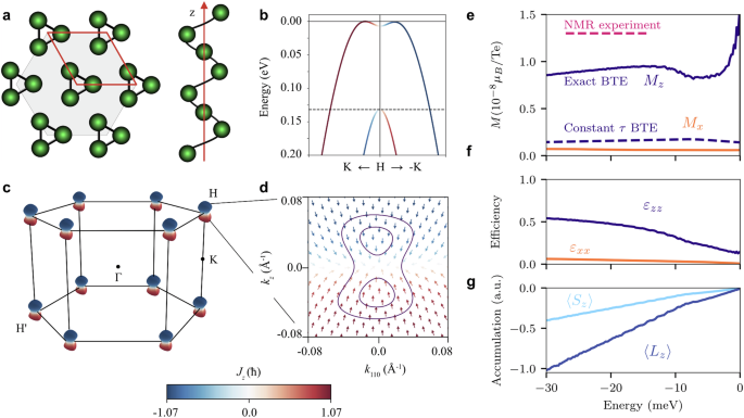
a Crystal structure of elemental Te. The helicity of an isolated chain along the z direction corresponds to right-handed Te. b Calculated valence band structure along the kz axis close to the H point in the Brillouin zone. The color encodes the z component of the total angular momentum. Its x and y components are much smaller in magnitude and are not shown. c The three-dimensional Fermi surface at E = −20 meV consists of six dumbbell-shaped hole pockets centered in the corners of the hexagonal Brillouin zone. d A single Fermi pocket at the H point projected onto a plane parallel to the z axis, where the arrows represent the total angular momentum directions. The constant energy contours at E = −5 meV (inner) and E = −20 meV (outer) are shown. e Current-induced magnetization Mz and Mx per Te atom induced by an electric current along the z and the x axis, respectively, (jx,z = 82 A cm−2) calculated for different chemical potential values. In the realistic doping region, the red dashed line indicates the induced magnetization estimated from NMR23. The solid lines represent our calculated values using exact solutions of the Boltzmann transport equations (BTE), while the dashed dark line shows the Mz value based on the relaxation time approximation21. f Charge-to-spin conversion efficiency vs chemical potential. g Spin and orbital contributions to angular momentum density without including g-factors.
Figure 2e shows the magnetization Mz induced by an electric current along the z axis ( jz = 82 A cm−2) as a function of the chemical potential, demonstrating good agreement with the NMR experimental data, which indicated Mz = 1.3 × 10⁻⁸μB per Te for this value of current23. We highlight a large improvement compared to the previous theoretical calculations, which underestimated the magnetization by an order of magnitude21,22,23. While one could presume a role of the orbital contribution, Fig. 2g shows that the orbital contribution alone only doubles the total magnetization for the wide range of chemical potentials that could result from the realistic hole doping levels. The magnetization Mz already incorporates the g-factors (2 for spin, 1 for orbital momentum), making the spin and orbital contributions nearly equal throughout the considered chemical potential range. The accuracy primarily comes from incorporating the k-state dependent relaxation time, achieved via the exact solution of the Boltzmann equation. Note that the observed magnetization increase near the valence band top is not fully reliable due to the division of two small numbers at very low hole populations in the magnetization defined in Eqs. (8), (9). Nevertheless, the spin accumulation exhibits the expected behavior at these small values of the chemical potential, as shown in Fig. 2g. Furthermore, an electric current along the x axis (jx = 82 A cm−2) induces magnetization Mx smaller than Mz by an order of magnitude, showing strong anisotropy relative to the screw axis. The temperature was set to T = 10 K for our calculations, but the results are similar at higher temperatures.
The remaining discrepancy between the experimental and theoretical values of Mz remains an important open question. In our analysis, we focus on how the accurate treatment of the relaxation times of individual carriers influences spin accumulation and its lifetime. Specifically, we calculate only the on-site orbital contribution to magnetization, commonly referred to in the literature as the atomic-centered approximation, while omitting intersite (or itinerant) contributions. To achieve more accurate predictions of magnetization, it is necessary to include additional factors, such as wavepacket self-rotation and corrections to the density of states in an applied magnetic field—both accounted for by the modern theory of orbital magnetization33,34,35,36. They are relevant for 5p orbitals, given their strongly delocalized nature in Te37, where previous studies suggested sizable contributions from wavepacket self-rotation38,39. Other extrinsic contributions to magnetization, such as from side-jump and skew scattering effects, become relevant only at higher hole densities38. These effects will be explored in more detail in future studies.
Although the induced magnetization is convenient for comparison with the NMR measurements, for nanodevices that rely on spin transport, the charge-to-spin conversion efficiency is a more important figure of merit. We define efficiency as:
$${\varepsilon }_{zz}=\frac{{\sum }_{{{\boldsymbol{k}}}}{\langle \, {\hat{J}}_{z}\rangle }_{{{\boldsymbol{k}}}}\delta {f}_{{{\boldsymbol{k}}}}}{{\sum }_{{{\boldsymbol{k}}}}| \delta {f}_{{{\boldsymbol{k}}}}| },$$
(10)
where \({\hat{J}}_{z}=({\hat{S}}_{z}+{\hat{L}}_{z})/J\) is the z component of the total angular momentum polarization operator, normalized with J = 3/2, and the electric field is applied along the z axis. Importantly, εzz has a transparent physical interpretation, resembling an intuitive efficiency definition (N↑ − N↓)/(N↑ + N↓), where Nσ is the non-equilibrium deviation of the total number of electrons with spin polarization σ. Whereas the numerator in Eq. (10) represents the total angular momentum polarization, its denominator quantifies the magnitude of the current-induced shift in the distribution function. In the quasi-classical picture, ∑k∣δfk∣ accounts for the induced imbalance between forward- and back-moving electron populations in momentum space. The efficiency is normalized from 0 to 1, where the former indicates no spin signal, and the latter describes the ideal situation of maximum accumulation with opposite spins of forward- and back-moving electrons.
Figure 2f shows the charge-to-spin conversion efficiency of Te calculated as a function of the chemical potential. Tellurium demonstrates exceptional efficiency, reaching 50% at realistic hole doping levels (7.4 × 10¹⁷/cm3) that correspond to the chemical potential of ~−20 meV22. This value is much higher than in most known materials with strong SOC40. We note that lower efficiencies of 20–40% have been recently reported for Te in the context of possible chirality-induced spin selectivity based on spin current calculations in a ballistic transport regime41,42. However, our approach is more suitable for sample sizes larger than the mean free electron path, as it considers nonballistic diffusive transport by including disorder.
Spin accumulation lifetime and relaxon spectra
We now examine the time dependence of spin accumulation by analyzing the relaxon spectrum. Figure 3 presents the spectral decomposition of the current-induced shift in the distribution function. When an electric current is applied along the z axis (see Fig. 3a), the spectrum has two pronounced peaks corresponding to collective relaxation modes: a fast mode with the relaxation rate Γ ≈ 0.5 and a slow mode with Γ ≈ 0.3 followed by a tiny satellite peak with Γ ≈ 0.22, as shown in Fig. 3c. The contributions to any observable from different collective relaxation modes can be independently calculated using the relaxon spectral decomposition in Eq. (6). For example, the average spin density is given by \({S}_{z}(t)={\sum }_{{{\boldsymbol{k}}}}{\langle {\hat{S}}_{z}\rangle }_{{{\boldsymbol{k}}}}\delta {f}_{{{\boldsymbol{k}}}}(t)/V={\sum }_{i}{\langle {\hat{S}}_{z}\rangle }_{i}{A}_{i}(t)\), where \({\langle {\hat{S}}_{z}\rangle }_{i}={\sum }_{{{\boldsymbol{k}}}}{\langle {\hat{S}}_{z}\rangle }_{{{\boldsymbol{k}}}}{{{\mathcal{V}}}}_{{{\boldsymbol{k}}}}^{i}/V\) is the spin polarization of the i-th relaxon.
Fig. 3: Current-induced spin accumulation in Te in the relaxon basis.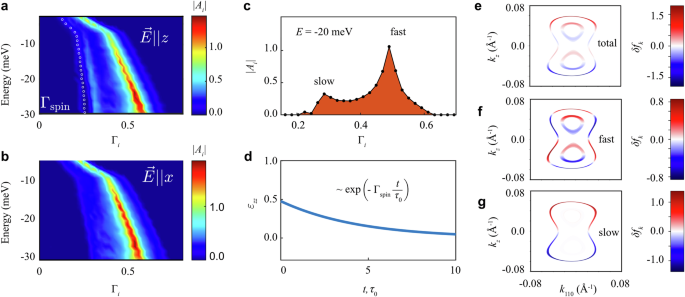
a, b Spectral decomposition at different values of chemical potential when an electric field \(\overrightarrow{E}\) is applied along the z and the x axis, respectively. The spectral amplitudes are color-coded, and white dots show the calculated spin relaxation rate. For \(\overrightarrow{E}\parallel z\) and energy E = −20 meV, c shows the spectrum, and d the spin density time dependence, normalized as charge-to-spin conversion efficiency. e The non-equilibrium deviation of the total distribution function δfk calculated near energies −5 meV (inner contour) and -20 meV (outer contour). f, g Contributions to δfk from relaxons with Γi > 0.33 and Γi
We find that the main contribution to Mz comes from the relaxons belonging to the slow modes (that is, Γi 3d). The resulting spin relaxation rate, marked by white dots in Fig. 3a, closely follows the slow relaxation modes, demonstrating their dominant role in governing spin accumulation. Conversely, when the electric current flows along the x axis (see Fig. 3b), the slow modes vanish. The low calculated current-induced magnetization Mx suggests that the fast mode corresponds to the mean electron scattering time, i.e., a normal relaxation mode.
To clarify the origin of the slow mode, we visualize δfk on the Fermi pockets near the H point. Figure 3e displays the −20 meV (and −5 meV) Fermi contours, where the color quantifies δfk. Figure 3f, g further isolate the fast and slow modes by calculating the contributions to δfk from relaxons with Γi > 0.33 and Γi E = −20 meV, the distribution δfk associated with the slow mode, where the spin polarization of induced holes is opposite to that of electrons, is identical to the angular momentum polarization pattern of electron states in Te (see Fig. 2d). This alignment of the slow mode distribution δfk with the spin polarization texture in k-space reduces back-scattering between the tips of the dumbbell-shaped pocket, thereby slowing this mode’s relaxation. Since nonmagnetic impurity scattering does not flip spin, the scattering probability \({W}_{{{{\boldsymbol{kk}}}}^{{\prime} }} \sim | \langle {{{\boldsymbol{k}}}}^{{\prime} }| {{\boldsymbol{k}}}\rangle {| }^{2}\) is diminishing when the states \(| {{\boldsymbol{k}}}\left.\right\rangle\) and \(| {{{\boldsymbol{k}}}}^{{\prime} }\left.\right\rangle\) have opposite spin polarizations. Nonetheless, the suppression is only partial because the spin polarization of the electron states is partial. The total angular momentum of these states never attains its maximum value of 3/2, as illustrated in Fig. 2d, in agreement with the angle-resolved photoemission spectroscopy (ARPES) results43. The contour at E = −5 meV shows a different scenario, where the slow mode is nearly absent in the spectral decomposition (see Fig. 3g), resulting in much smaller current-induced accumulation (Fig. 2g) and shorter spin lifetime (Fig. 3a).
The spin relaxation mechanism in Te is particularly interesting. Notably, the conventional Dyakonov-Perel mechanism44 is negligible in this context. Interband transitions, which could otherwise contribute to spin relaxation within coherent dynamics, are suppressed due to the large band splitting (≈100 meV) compared to other energy scales in the system. As a result, coherent spin relaxation processes can, to a first approximation, be ignored in Te. As spin relaxation in Te arises from collisions with nonmagnetic impurities, it resembles the Elliot-Yafet mechanism45,46 and can be thought of as a generalization of this mechanism for materials with strong SOC. In chiral Te, the strong SOC introduces significant mixing of opposite spin states in Bloch electrons, which would typically reduce spin lifetime. Yet, this suppression is counterbalanced by the strong spin and orbital polarization of carriers near the H point (see Fig. 2a–d and Supplementary Fig. 1). The structural chirality of Te imprints this polarization onto wavefunctions, aligning electrons velocities with their spin polarizations. This spin protection mechanism, stemming from the suppressed back-scattering of spin-polarized states, bears the closest resemblance to the behavior of protected edge states in graphene47 and topological insulators48. This analogy makes it promising to study quantum-geometrical aspects49,50 of spin accumulation and its lifetime in chiral materials such as Te51,52,53, especially in light of recently observed in ARPES experiments in-gap states54 that are similar to the robust bound states localized at the chain boundaries in the Su-Schrieffer-Heeger model55.
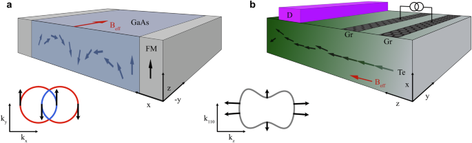
These observations suggest that the generated spin accumulation can propagate over long distances. The spin diffusion length is approximately the product of the spin relaxation time and the Fermi velocity. In Te, it is estimated to be about three times the mean free path (see Fig. 3a). Recent magnetoresistance experiments on Te nanoflakes reported mean free paths of 22–34 nm56, corresponding to spin diffusion lengths of 66–102 nm. This range is comparable to the phase coherence and the spin-orbit relaxation lengths, which reach up to 100 nm based on weak localization model calculations. Such spin diffusion length scales are promising for crafting efficient spintronic devices that make use of non-local spin transport in two-dimensional heterostructures based on Te thin films or tellurene. A potential all-electrical spintronic device could operate in a non-local spin diffusive regime: in the ‘injector’ region, an electric current along the chain induces parallel magnetization, and in the ‘conductor’ region, spin accumulation diffuses over hundreds of nanometers towards the ‘detector’ region, where the spin signal is measured through spin-to-charge conversion (see Fig. 1b).
However, a direct mapping between relaxon lifetimes and experimental transport coefficients remains an open question for future research. Based on the mean free path (≈30 nm) and the Fermi velocity (≈ 30 nm/ps), we estimate the mean scattering time to be ~1 ps, a typical value for semiconductors. This suggests that the spin relaxation time in Te would be ~3 ps, which is significantly shorter than the typical Dyakonov-Perel and Elliot-Yafet timescales in III-V semiconductors57,58, ranging from 10 to 100 ps at similar high carrier densities (1016−1018 cm−3), and than that extending up to nanoseconds in GaAs quantum wells that host PSH10.
Finally, we highlight a noticeable correlation between slow relaxons and charge-to-spin conversion efficiency. Long-living relaxons contribute more to the distribution function and, consequently, to magnetization, as indicated by the linear τ-dependence of relaxon amplitudes in Eq. (7). The slow relaxons, with lifetimes around 3τ0, carry spin and angular momentum, leading to a threefold enhancement in magnetization compared to the constant relaxation time approximation. However, Eq. (7) also includes the relaxon eigenvector, which introduces a correction to our estimate due to the complex spectrum of relaxons. This spectrum contains two peaks representing collective relaxation modes, which resemble relaxon wavepackets. Unlike previous studies, our reported order-of-magnitude magnetization enhancement comes from accounting for the exact amplitudes, shapes, and widths of these wavepackets, as captured by the exact mapping of the initial distribution function onto the relaxon basis. Remarkably, the charge-to-spin conversion efficiency is amplified by the high spectral density of spin-carrying slow relaxons. This efficiency is mainly determined by the ratio of spectral weights between the slow and fast wavepackets. Thus, to maximize the efficiency, it is crucial to identify materials that host slower relaxons with higher spectral amplitudes, a key avenue for future research.