Principle of HO MINFLUX
Conventional MINFLUX generally utilizes a first-order vortex beam as the doughnut excitation, which is a special type of Laguerre-Gaussian (LG) beam23. The amplitude profile of a Laguerre Gaussian beam is given by
$${\varphi }_{lp}({\boldsymbol{r}})=\sqrt{\frac{2p!}{\pi (p+|l|)!}}\frac{1}{w}{\left(\frac{\sqrt{2}r}{w}\right)}^{|l|}{L}_{p}^{|l|}\left(\frac{2{r}^{2}}{{w}^{2}}\right){e}^{-\frac{{r}^{2}}{{w}^{2}}}{e}^{-il\theta }$$
(1)
where \({\boldsymbol{r}}\,=\,(r,\theta )\) is the position vector in the polar coordinate system, l and p are the azimuthal and radial indices, respectively. w is the radius of beam waist, which is related to the full width at half maximum (FWHM) as \(\text{FWHM}=\sqrt{2\,\mathrm{ln}\,2}w\). \({L}_{p}^{|l|}(\bullet )\) is the associated Laguerre polynomial.
When \(l\,\ne\, 0\), the LG beam exhibits vortex phase front and carries orbital angular momentum (OAM)24,25, where the center of the beam appears as the singularity, presenting a doughnut-like profile. The order of vortex is determined by the azimuthal index l, also known as the topological charge. l = 1 refers to the most widely applied doughnut beam. The radial index p brings more oscillations to the beam profile. As the region of interest (ROI) of MINFLUX is typically much smaller than the beam width, the p index has negligible effect on the beam profile as well as the precision of MINFLUX, as will be elaborated on later. Therefore, in this study, we mainly focus on cases that p = 0.
The intensity profile of an l-order vortex beam is described by
$$I({\boldsymbol{r}})\propto {\left(\frac{2{r}^{2}}{{w}^{2}}\right)}^{|l|}{e}^{-\frac{2{r}^{2}}{{w}^{2}}}$$
(2)
As can be noted, in the vicinity of central region, \(I({\boldsymbol{r}})\propto {r}^{2|l|}\), which behaves similarly to the PSF of \(|l|\)-photon fluorescence when using a first-order vortex beam. Thus, while multiphoton excitation has been shown to improve the localization precision of MINFLUX19,21, HO vortex-based MINFLUX achieves comparable performance and offers a more convenient implementation, requiring only the modulation of the excitation wavefront.
The enhancement of localization precision with HO vortex beams can be intuitively illustrated by the sensitivity of photon detection on the position, or the propagation of uncertainty from photon detection to position estimation, as is shown in Fig. 1. Considering the arrival of photons follows a Poisson process, the Poisson rate \(\lambda\), which represents the mean photon count, is proportional to the excitation intensity, \(\lambda \propto I(r)\). We can then derive that
$$\frac{\partial \lambda }{\partial r}=\frac{2\lambda }{r}\left(|l|-\frac{2{r}^{2}}{{w}^{2}}\right)$$
(3)
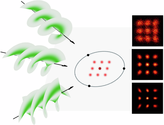
Fig. 1: Enhanced localization precision with HO vortex beams.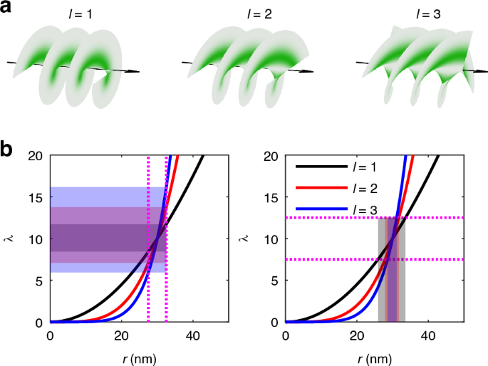
a Helical wavefronts of vortex beams with different orders. b Illustration of enhanced sensitivity (left) and reduced uncertainty (right) achieved using HO vortex excitation. Shaded regions represent the variations in \(\lambda (r)\) with respect to \(r(\lambda )\). Beam radius w is set to 300 nm
Near the center where \(r\ll w\), we have \(\frac{\partial \lambda }{\partial r}\approx \frac{2\lambda }{r}|l|\). Consequently, given the same position \(r\) and Poisson rate \(\lambda\), the photon counts detected in HO vortex are more sensitive to the variation of position. Regarding the propagation of uncertainty, with the same uncertainty in photon detection, the uncertainty in position estimation is decreased for HO vortex beam. For an l-order vortex beam, there is an \(|l|\)-fold increase in the sensitivity and decrease in the uncertainty, which enhances the performance in localization microscopy.
Localization precision analysis
To see how the order of vortex beams exactly affects the MINFLUX precision of localization, we analyze the Cramér-Rao Bound (CRB) for different order vortex beams and the effect of some other practical parameters, such as the length of TCP L and the signal to background ratio (SBR).
Generally, two common TCPs are employed in MINFLUX: the widely used four-point TCP and the raster scan TCP, as illustrated in Fig. 2a. We therefore examine both configurations for comparison.
Fig. 2: Performance of MINFLUX with HO vortex beam.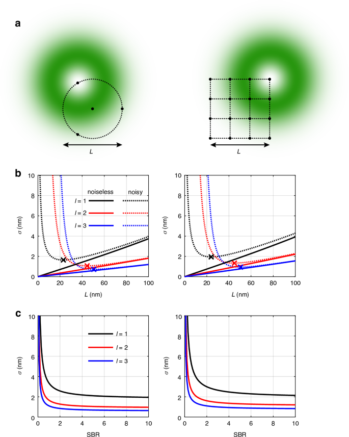
a The four-point TCP and raster scan TCP. b Central CRB plotted as a function of L. For noisy cases, SBR is set as 4 at L = 50 nm. c Central CRB plotted as a function of the SBR, where \(L={\rm{50nm}}\). The total photon count is set as 100
The analytical expression for the CRB of MINFLUX is typically complex, influenced by the illumination pattern, the TCP and the position of the emitter, see Method for the detailed derivations. For conventional MINFLUX with four-point TCP, an explicit expression can be derived for the central CRB as
$${\sigma }_{{\bf{0}}}=\frac{L}{2n\sqrt{2N}}\frac{s}{|l|-\frac{{L}^{2}}{2{w}^{2}}}$$
(4)
Here n stands for the n-photon excitation, l refers to the order of vortex beam, N is the number of detected photons and \(s=\sqrt{(1+\frac{3}{4\text{SBR}})(1+\frac{1}{\text{SBR}})}\). Equation (4) is a generalization of Eq. (2) in Ref. 19. Apparently, the order l improves the central CRB slightly more than \(|l|\)-fold, as L is much smaller than w. Vortex order l thus plays a similar role as n, requiring only \(1/{l}^{2}\) of the photons to achieve the same precision as a first order doughnut beam. The excitation wavelength primarily influences the precision of MINFLUX by affecting the focused beam size w, which has a negligible impact in the subdiffraction region, as studied in Ref.4,19.
To facilitate a comparison between MINFLUX and RASTMIN, we numerically calculate the CRB for both TCPs. Figure 2b illustrates the central CRB as a function of L. In the excess noise-free scenario represented by the solid curves, the CRB always decreases as L reduces, with higher-order vortex beams consistently yielding smaller CRBs. In this ideal case, higher-order vortices always achieve superior precision given the same L. For noisy scenarios, as represented by the dashed curves, the presence of background noise significantly affects the localization precision of MINFLUX, as the signal can be overwhelmed by the noise near the center. Consequently, continuously decreasing L gives rise to a very low SBR, which may lead to a dramatic increase in the CRB. An optimal L which minimizes the CRB can be identified for each vortex beam, as indicated by the crosses on the dashed lines in Fig. 2b. The minimum CRBs achieved under MINFLUX for l = 1, 2, and 3 are 1.64 nm, 1.06 nm, and 0.72 nm, respectively, while under RASTMIN, the corresponding values are 1.95 nm, 1.34 nm, and 0.94 nm, respectively. For both TCPs, higher-order vortices deliver superior optimal precisions.
It should be noted that the SBR for HO vortex beams is more sensitive. For instance, in MINFLUX, the relation between SBR and L is given by
$${\rm{SBR}}_{L}={\text{SBR}}_{{L}_{0}}{\left(\frac{L}{{L}_{0}}\right)}^{2|l|}{e}^{-\frac{{L}^{2}-{L}_{0}^{2}}{2{w}^{2}}}$$
(5)
where the SBR decreases more rapidly for HO vortex beams as L reduces. Therefore, at small L, HO vortex beams may result in even larger errors due to the extremely low SBR.
Figure 2c analyzes the effect of SBR, where the length of TCP is set to be 50 nm. It is evident that when the SBR is too low (e.g. SBR
While in both MINFLUX and RASTMIN, HO vortex beams improve the maximum precision at the center, MINFLUX with four-point TCP offers superior improvement. For example, with L = 50 nm, SBR = 4, central CRB values under MINFLUX for l = 1, 2, 3 are 2.31 nm, 1.15 nm and 0.76 nm, respectively. This improvement slightly exceeds l-fold, as can also be inferred from Eq. (4). In RASTMIN, the corresponding values are 2.66 nm, 1.44 nm, and 1.00 nm, showing a smaller improvement on the central CRB compared to MINFLUX. Compared with several variants of MINFLUX which have demonstrated nanometer-scale resolution (as summarized in the table in Ref.26), HO vortex beams hold significant promise for further improving MINFLUX precision to the sub-nanometer level under optimized conditions.
While MINFLUX excels in achieving higher central precision, RASTMIN offers advantages with its expanded FOV. In Fig. 3a, we study the CRB distribution across two-dimensional (2D) space. As can be observed, for MINFLUX, increasing the vortex order significantly reduces the central CRB, but this improvement is limited to the central region. The CRB deteriorates considerably outside the central area, indicating that optimal localization requires confining the emitter near the center of the TCP. In contrast, RASTMIN, despite its slightly inferior central CRB compared to MINFLUX, enhances the CRB more uniformly across the entire FOV, accommodating a larger region for the emitter. Therefore, MINFLUX is particularly well-suited for an iterative scan scheme, which progressively confines the emitter towards the center of the TCP, while RASTMIN is more effective with a fixed scan scheme, providing a larger FOV for tracking emitters over extended areas. Figure 3b plots the CRB along 0 degree for different orders of vortex beams. In MINFLUX, the CRB improves significantly with HO vortex beams when the emitter is near the central region. However, the precision may even drop below that of lower-order beams when the emitter deviates further from the center. For RASTMIN, the CRB is improved for HO vortex within the entire FOV. Additionally, the increase in CRB from the center to the edge is slower in RASTMIN compared to MINFLUX, indicating more uniform performance across the FOV.
Fig. 3: The CRB for vortex beams with order l = 1, 2, 3.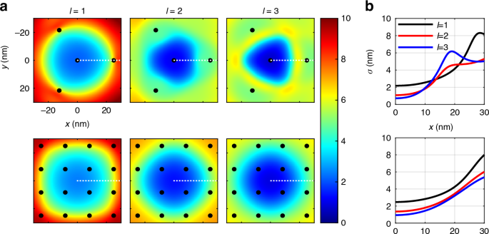
a CRB distribution over 2D space. b Variation of CRB along x axis as indicated by the dashed lines in a. Top: four-point TCP. Bottom: raster scan TCP. Parameter setting: N = 100, L = 50 nm, SBR = 4
Define the effective FOV (EFOV) as the circular area where the CRB is below 4 nm, a threshold chosen to represent high-precision localization capabilities. Under this definition, we quantify the EFOV for different orders of vortex beams in both MINFLUX and RASTMIN. For MINFLUX, the diameter of EFOV is 35.85 nm for l = 1, 32.80 nm for l = 2, and decreases to 29.19 nm for l = 3. For RASTMIN, the EFOV shows an evident increase, from 37.88 nm for l = 1, to 42.80 nm for l = 2, and 45.93 nm for l = 3. These data intuitively show that increasing the vortex order l significantly expands the EFOV in RASTMIN, suggesting the potential for imaging larger areas with high precision, which could be particularly beneficial for studying extended cellular structures or dynamic processes over wider regions.
In practice, prior information about emitter’s position is often available through approaches such as wide-field imaging, preliminary confocal scans, or initial rounds of conventional MINFLUX. Under such conditions, the Bayesian CRB27,28 can be used to evaluate the precision of localization. Typically, prior information yields a normal distribution for the emitter’s position29. Assuming a standard deviation of 50 nm for the prior distribution, the Bayesian CRB for MINFLUX is calculated to be 6.95 nm, 4.59 nm, 3.63 nm for l = 1, l = 2, and l = 3, respectively. For RASTMIN, the corresponding values are 7.22 nm, 4.80 nm, and 3.81 nm. Both cases show that the precision conditioned on prior information can be significantly improved with HO vortex beams.
Besides the improved precision, another advantage of HO vortex beams lies in their enhanced robustness within turbid scattering media, such as biological tissues. As demonstrated in previous works30,31, higher-order vortex beams exhibit higher transmittance in strongly scattering environments, enabling them to penetrate deeper into biological tissues. This property further enhances the capability of HO vortex beams for deep in vivo biological observations.
The effect of radial index
In the previous section, we examined the performance of MINFLUX for the case where p = 0. Here, we show that the radial index p has a negligible effect on the localization precision of MINFLUX.
According to Eq. (1), the radial index p influences the beam profile via the associated Laguerre polynomial. Since the ROI in MINFLUX is typically much smaller than the beam width, the leading term of the associated Laguerre polynomial in this case is a constant. As a result, the profile of the beam within the ROI is not significantly affected by the radial index, which in turn subtly impacts the localization precision of MINFLUX.
In Fig. 4, we numerically calculate the central CRB for vortex beams with different radial indices. It is apparent that for both MINFLUX and RASTMIN, beams with the same azimuthal index (solid and dashed curves) yield nearly identical CRB values, irrespective of the radial index. Noticeable divergence in CRB values emerges when the length of the TCP is excessively large, and this divergence reduces as the azimuthal index l increases. The 2D CRB map for different radial indices is presented in Supplementary Section I, where it is also observed that the CRB within the entire ROI changes little with varying p indices.
Fig. 4: The effect of radial index on the central CRB.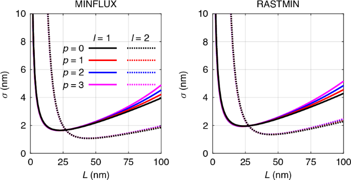
Left: MINFLUX. Right: RASTMIN. Different line styles represent different l index, while different colors denote different p index. Parameter setting: N = 100, SBR = 4
Monte Carlo simulation
To verify our theoretical analysis and demonstrate the performance of HO vortex-based MINFLUX, we employ Monte Carlo simulation method to simulate the localization process in MINFLUX. We generate multinomial random numbers to represent photon counts at each scanning point, corresponding to the probability distribution over the TCP. Subsequently, we apply maximum likelihood estimation (MLE) to retrieve the emitter’s position. The estimator used in MLE is given by
$${\hat{{\boldsymbol{r}}}}_{e}=\mathop{\text{arg}\,\max }\limits_{{{\boldsymbol{r}}}_{e}}P({\boldsymbol{n}}|{{\boldsymbol{r}}}_{e})$$
(6)
Details refer to Methods section. We conduct Monte Carlo simulations for both MINFLUX and RASTMIN using different orders of vortex beams, with results summarized in Fig. 5. The sample considered here is a 3 × 3 array of emitters, which can be realized using fluorophore-labeled DNA origami. The distance between adjacent emitters is 5 nm. In each trial, we set the total photon number N to 300, the length of TCP L to 50 nm, and the SBR to 4. For each case, 2000 trials are performed to evaluate the root mean square error (RMSE), which is defined as
$${\text{RMSE}}=\sqrt{\frac{1}{2}{\rm{E}}({|{{\hat{\boldsymbol{r}}}}_{e}-{{\boldsymbol{r}}}_{e}|}^{2})}$$
(7)
where the factor 2 is to keep consistency with the arithmetic mean of CRB in Eq. (16).
Fig. 5: Simulated results for HO vortex based MINFLUX localization.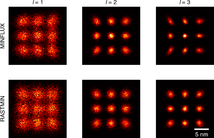
Top: MINFLUX, bottom: RASTMIN. Scale bar: 5 nm. Simulation conditions: N = 300, L = 50 nm, SBR = 4, trials = 2000
The results demonstrate that HO vortex beams significantly enhance the resolvability of the emitters, achieving substantially smaller estimation errors compared to conventional MINFLUX. The average localization error decreases from 1.33 nm (l = 1) to 0.75 nm (l = 2) and 0.59 nm (l = 3). Comparable improvements are observed in RASTMIN, with the average error reduced from 1.52 nm to 0.88 nm and 0.64 nm, respectively. The simulations also validate the effectiveness of the CRB derived in this study. The overall RMSEs for all cases remain within 5% of the theoretical bounds, illustrating that the localization precision is well-bounded by the CRB.
Additionally, as originally noted by Balzarotti et al.4, the localization precision is not isotropic in 2D space. Our simulations also reveal that the estimated positions are not isotropically distributed along each direction when the emitter is not at the center of TCP. While the estimated positions generally follow bivariate Gaussian distributions, their standard deviations along orthogonal axes are typically unequal, except for the central emitter. This anisotropy becomes more noticeable with the use of HO vortex beams, particularly in MINFLUX. For instance, in 3rd-order MINFLUX, the estimated positions of edge emitters exhibit strong anisotropy. The results in RASTMIN also indicate anisotropy, although the effect is less pronounced compared to MINFLUX. A detailed analysis of the anisotropy of CRB is provided in Supplementary Section II.