Phonon BTE
The phonon BTE describes the evolution of phonon distributions over time in a system. For a system with a heat source at steady state, the energy-based phonon BTE under the single mode relaxation time approximation can be expressed as66,60:
$${\boldsymbol{v}}\cdot \nabla e=\frac{e-{e}^{0}}{\tau }+Q,$$
(1)
where e(x, s, ω, p) is the phonon energy distribution function, which depends on spatial position x, directional unit vector s, phonon frequency ω, and phonon branch p. v(ω, p) is the group velocity, and τ(ω, p) is the relaxation time, which can be obtained for all phonons at different ω and p using first-principles Density Functional Theory (DFT) calculations. Q represents the volumetric heat source intensity, and e0(x) is the equilibrium part of the distribution function. According to energy conservation, e0 is related to e through67:
$${e}^{0}=\frac{1}{4\pi }C{T}_{L},$$
(2)
$${T}_{L}=\frac{{\int}_{4\pi }{\sum }_{p}{\int}_{\omega }\frac{e}{\tau }d\omega d\Omega }{{\sum }_{p}{\int}_{\omega }\frac{C}{\tau }d\omega },$$
(3)
where C(ω, p) is the volumetric heat capacity for a given phonon mode, TL is the lattice temperature, and Ω is the solid angle in spherical coordinates. The heat flux can be calculated by:
$${\bf{q}}={\int}_{4\pi }\sum _{p}{\int}_{\omega }{\bf{v}}ed\omega d\Omega .$$
(4)
Boundary conditions
For the JAX-BTE solver, three built-in boundary conditions commonly used in phonon BTE simulations57,58 are implemented.
Isothermal boundary
This boundary absorbs all incoming phonons and emits phonons in thermal equilibrium at a specific temperature T back into the simulation domain. This can be described as:
$$e\left({{\boldsymbol{x}}}_{b},{\boldsymbol{s}},\omega ,p\right)=\frac{C}{4\pi }T,\,{\boldsymbol{s}}\cdot {{\boldsymbol{n}}}_{b} \,
(5)
where xb is the position at the boundary and nb is the outward-pointing normal unit vector at the boundary.
Diffusely reflecting boundary
This adiabatic boundary reflects phonons leaving the simulation domain with equal probability in all possible directions pointing into the simulation domain. According to energy conservation, it is represented as:
$$e\left({{\boldsymbol{x}}}_{b},{\boldsymbol{s}},\omega ,p\right)=\frac{1}{\pi }{\int}_{{{\boldsymbol{s}}}^{{\prime} }\cdot {{\boldsymbol{n}}}_{b}\ > \ 0}e\left({{\boldsymbol{x}}}_{b},{{\boldsymbol{s}}}^{{\prime} },\omega ,p\right)\left\vert {{\boldsymbol{s}}}^{{\prime} }\cdot {{\boldsymbol{n}}}_{b}\right\vert d\Omega ,\,{\boldsymbol{s}}\cdot {{\boldsymbol{n}}}_{b}\,
(6)
where \({{\boldsymbol{s}}}^{{\prime} }\) are all angles that point out of the domain and the use of this boundary condition implies a rough surface.
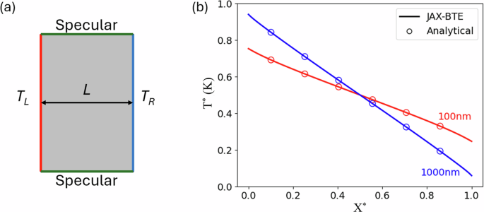
Specularly reflecting boundary
Another adiabatic boundary condition, specular reflecting boundaries assumes phonons reflect as if from a mirror, where the phonon energy along the reflected angle is equal to that of the incident angle:
$$e\left({{\boldsymbol{x}}}_{b},{\boldsymbol{s}},\omega ,p\right)=e\left({{\boldsymbol{x}}}_{b},{{\boldsymbol{s}}}^{{\prime} },\omega ,p\right),\,{\boldsymbol{s}}\cdot {{\boldsymbol{n}}}_{b}\,
(7)
where \({{\boldsymbol{s}}}^{{\prime} }={\boldsymbol{s}}-2{{\boldsymbol{n}}}_{b}({\boldsymbol{s}}\cdot {{\boldsymbol{n}}}_{b})\) is the reflected phonon direction. This boundary condition assumes a perfectly smooth surface.
Band discretization
For discretizing phonon energy in the frequency and polarization domains, the wave vector space is divided into n equidistant intervals [K0, …, Kn], referred to as bands, where K0 is the minimum wave vector and Kn is the maximum wave vector. For each wave vector interval, phonon properties such as heat capacity, relaxation time, and group velocity are calculated by weighted averaging these properties within the interval (i.e., within each band). Specifically, for each band, the representative phonon properties are given by63,68:
$${C}_{\lambda }=\mathop{\sum }\limits_{k > {K}_{n-1}}^{{K}_{n}}C,$$
(8)
$${{\boldsymbol{v}}}_{\lambda }=\frac{\mathop{\sum }\nolimits_{k\ > \ {K}_{n-1}}^{{K}_{n}}C{\boldsymbol{v}}}{\mathop{\sum }\nolimits_{k\ > \ {K}_{n-1}}^{{K}_{n}}C},$$
(9)
$${\tau }_{\lambda }=\frac{\mathop{\sum }\nolimits_{k\ > \ {K}_{n-1}}^{{K}_{n}}C{v}^{2}\tau }{{{\boldsymbol{v}}}_{\lambda }\mathop{\sum }\nolimits_{k\ > \ {K}_{n-1}}^{{K}_{n}}Cv},$$
(10)
$${Q}_{\lambda }=\frac{{C}_{\lambda }Q}{{\sum }_{\lambda }{C}_{\lambda }},$$
(11)
where λ is the index of the phonon band and k is the wave vector. The original integral equation of frequency is transformed into a summation form:
$$\mathop{\sum}\limits_{p}{\int}_{\omega }\frac{e}{\tau }d\omega =\mathop{\sum}\limits_{\lambda }\frac{{e}_{\lambda }}{{\tau }_{\lambda }}\,,$$
(12)
$$\mathop{\sum}\limits_{p}{\int}_{\omega }\frac{C}{\tau }d\omega =\mathop{\sum}\limits_{\lambda }\frac{{C}_{\lambda }}{{\tau }_{\lambda }}\,.$$
(13)
Angle discretization
The angle discretization transforms the integration over directional space into a weighted summation35,57:
$${\int}_{4\pi }{e}_{\lambda }d\Omega =\mathop{\int}\nolimits_{0}^{\pi }\mathop{\int}\nolimits_{0}^{2\pi }{e}_{\lambda }sin\theta d\theta d\varphi =\sum _{\alpha }{\beta }_{{\theta }_{\alpha }}{\beta }_{{\varphi }_{\alpha }}sin{\theta }_{\alpha }{e}_{\alpha ,\lambda }=\sum _{\alpha }{\beta }_{\alpha }{e}_{\alpha ,\lambda }.$$
(14)
Here θ is the polar angle and φ is the azimuthal angle. α is the index for the sampled direction sα = (cosθ, sinθcosφ, sinθsinφ). The weights \({\beta }_{{\theta }_{\alpha }}\) and \({\beta }_{{\varphi }_{\alpha }}\), as well as their corresponding directions, are calculated using Gauss-Legendre quadrature to achieve high numerical accuracy with reduced computational cost. The final weight of the phonon energy in direction α and band λ, eα,λ, is given as \({\beta }_{\alpha }={\beta }_{{\theta }_{\alpha }}{\beta }_{{\varphi }_{\alpha }}sin{\theta }_{\alpha }\).
Spatial discretization
After applying band and angular discretization, the phonon BTE in its steady-state form becomes:
$${{\boldsymbol{v}}}_{\lambda }\cdot \nabla {e}_{\alpha ,\lambda }=-\frac{{e}_{\alpha ,\lambda }-{e}_{\lambda }^{0}}{{\tau }_{\lambda }}+{Q}_{\lambda }$$
(15)
where λ is the index of the band and α is the angle index. The equilibrium energy is represented by:
$$\begin{array}{l}{e}_{\lambda }^{0}=\frac{1}{4\pi }{C}_{\lambda }{T}_{L},\\ {T}_{L}=\frac{{\sum }_{\lambda }{\sum }_{\alpha }{\omega }_{\alpha }\frac{{e}_{\alpha ,\lambda }}{{\tau }_{\lambda }}}{{\sum }_{\lambda }\frac{{C}_{\lambda }}{{\tau }_{\lambda }}}.\end{array}$$
(16)
The finite volume method (FVM) is employed to spatially discretize the equation. Namely, by dividing the computational domain into discrete control volumes (cells), and the equation is solved by balancing the energy fluxes across the boundaries of each control volume. The governing equation is integrated over the volume of each cell, transforming the spatial derivative into surface integrals across the cell faces. For a control volume i, the discretized form of the BTE becomes,
$$\sum _{j\in N(i)}{{\boldsymbol{v}}}_{i,\lambda }\cdot {{\boldsymbol{n}}}_{ij}{S}_{ij}{e}_{ij,\alpha ,\lambda }=-\frac{{e}_{i,\alpha ,\lambda }-{e}_{i,\lambda }^{0}}{{\tau }_{i,\lambda }}{V}_{i}+{Q}_{i,\lambda }{V}_{i},$$
(17)
where Vi is the volume of the cell i and N(i) is the list of neighboring cells of cell i, Sij is the area of the interface between cell i and cell j, nij is the outward-facing normal vector at the interface, and eij,α,λ is the phonon energy at the interface, which is computed using upwind scheme to ensure numerical stability,
$${e}_{ij,\alpha ,\lambda }={e}^{{\prime} }+\nabla {e}^{{\prime} }\cdot {d}_{ij}^{{\prime} },$$
(18)
where \({e}^{{\prime} }\) and \(\nabla {e}^{{\prime} }\) are the phonon energy density and its gradient in the cell from the upwind direction (s ⋅ n > 0), while \({d}_{ij}^{{\prime} }\) is the vector from the center of the upwind cell to the center of interface ij. The gradient \(\nabla {e}^{{\prime} }\) is numerically computed using the Green-Gauss method.
Directly solving the full system of algebraic equations (Eq. (17)) is computationally challenging and unstable due to the presence of the equilibrium energy term, which is a function of the integral of the phonon energy distribution across all directions and bands. To address this, the system is solved iteratively with pseudo-time stepping. Namely, at each iteration (i.e., pseudo-time step) n + 1, the phonon energy distribution is updated based on the changes (or increments) from the previous iteration n. As a result, Eq. (17) can be reformulated in its incremental form,
$$\frac{{\Delta }{e}_{i,\alpha ,\lambda}^{n+1}}{{\tau}_{i,\lambda}}+\frac{1}{{V}_{i}}\sum _{j\in N\left(i\right)}\Delta {e}_{ij,\alpha ,\lambda }^{n+1}{{\boldsymbol{v}}}_{i,\lambda }\cdot {{\boldsymbol{n}}}_{ij}{S}_{ij}=-\frac{1}{{V}_{i}}\sum _{j\in N\left(i\right)}{e}_{ij,\alpha ,\lambda }^{n}{{\boldsymbol{v}}}_{i,\lambda }\cdot {{\boldsymbol{n}}}_{ij}{S}_{ij}-\frac{{e}_{i,\alpha ,\lambda }^{n}-{e}_{i,\lambda }^{n,0}}{{\tau }_{i,\lambda }}+{Q}_{i,\lambda }$$
(19)
where Δen+1 = en+1 − en is the incremental update of phonon energy density between iterations. This incremental form allows for gradual convergence towards the steady-state solution, ensuring numerical stability and avoiding sharp changes in the solution.
Iterative matrix formulation and solution scheme
Once the element-wise algebraic equations (19) for the discretized BTE have been established, it is advantageous to express these equations in matrix form. Each cell-wise equation can be represented as a linear combination of the unknown phonon energy difference Δen, leading to a system of linear equations for all cells under each band-angle combination. This matrix representation facilitates the use of GPU computing, enabling batch processing of the equations and significantly accelerating the simulation. Specifically, the matrix form is expressed as follows:
$${{\boldsymbol{A}}}_{\alpha ,\lambda }\Delta {e}_{\alpha ,\lambda \,}^{n+1}={{\boldsymbol{b}}}_{\alpha ,\lambda }^{n},$$
(20)
where Aα,λ is the stiffness matrix for angle α and band λ, which has the dimensions of Nc × Nc, with Nc being the total number of cells. The diagonal and off-diagonal elements of the matrix are given by:
$$\begin{array}{l}{A}_{ii,\alpha ,\lambda }=\frac{1}{{\tau }_{i,\lambda }}+\mathop{\sum}\limits_{j\in N\left(i\right)}\frac{1}{{V}_{i}}{{\boldsymbol{v}}}_{i,\lambda }\cdot {{\boldsymbol{n}}}_{ij}H\left({{\boldsymbol{v}}}_{i,\lambda }\cdot {{\boldsymbol{n}}}_{ij}\right){S}_{ij},\\ {A}_{ij,\alpha ,\lambda }=\frac{1}{{V}_{i}}{{\boldsymbol{v}}}_{i,\lambda }\cdot {{\boldsymbol{n}}}_{ij}H\left({-{\boldsymbol{v}}}_{i,\lambda }\cdot {{\boldsymbol{n}}}_{ij}\right),\end{array}$$
(21)
where H(⋅) is the Heaviside step function. The right-side vector bn is expressed as:
$$\begin{array}{ll}{b}_{i,\alpha ,\lambda }^{n}=-\mathop{\sum}\limits_{j\in N\left(i\right)}\frac{1}{{V}_{i}}{{\boldsymbol{v}}}_{i,\lambda }\cdot {{\boldsymbol{n}}}_{ij}H\left({{\boldsymbol{v}}}_{i,\lambda }\cdot {{\boldsymbol{n}}}_{ij}\right){S}_{ij}\left({e}_{i,\alpha ,\lambda }^{n}+\nabla {e}_{i,\alpha ,\lambda }^{n}\cdot {{\boldsymbol{d}}}_{i,ij}\right)\\ \qquad\quad\,\,\,-\mathop{\sum}\limits_{j\in N\left(i\right)}\frac{1}{{V}_{i}}{{\boldsymbol{v}}}_{i,\lambda }\cdot {{\boldsymbol{n}}}_{ij}H\left({-{\boldsymbol{v}}}_{i,\lambda }\cdot {{\boldsymbol{n}}}_{ij}\right){S}_{ij}\left({e}_{j,\alpha ,\lambda }^{n}+\nabla {e}_{j,\alpha ,\lambda }^{n}\cdot {{\boldsymbol{d}}}_{j,ij}\right)\\ \qquad\quad\,\,\,-\frac{{e}_{i,\alpha ,\lambda }^{n}}{{\tau }_{i,\lambda }}+\frac{{e}_{i,\alpha ,\lambda }^{n,0}}{{\tau }_{i,\lambda }}+{Q}_{i,\lambda }.\end{array}$$
(22)
In these equations, the stiffness matrix Aα,λ depends only on material properties and mesh topology, and thus remains unchanged throughout the simulation process. The vector \({{\boldsymbol{b}}}_{\alpha ,\lambda }^{n}\), however, needs to be re-evaluated at each iteration after updating the phonon energy density. To solve the linear system, the bi-conjugate gradient (Bi-CG) method is employed, with a Jacobi preconditioner to improve convergence.
In the iterative solver, the initial phonon energy density is calculated based on the given initial temperature. For each iteration, both the equilibrium energy density and phonon energy density are updated using equation (3). The complete solution procedure is summarized as follows60:
-
1.
Set initial equilibrium energy density e0 and phonon energy density e according to the initial temperature.
-
2.
Solve the discretized form of the BTE according to the input boundary conditions to update phonon energy density e according to equation (19).
-
3.
Update e0 and T based on equation (16).
-
4.
Repeat step 2 and 3 until converge is achieved when the following criteria are satisfied,
$$\begin{array}{rlr}{\epsilon }_{T}&=\sqrt{\mathop{\sum }\limits_{i}^{N}\frac{{\left({T}_{i}^{n}-{T}_{i}^{n+1}\right)}^{2}}{N}}/{T}_{max}
(23)
where N is the number of spatial cells, \({\tilde{\epsilon }}_{T}\) and \(\tilde{{\epsilon }_{q}}\) are user-defined target temperature residual and heat flux residual, repsectively.
Forward and inverse modeling workflow
The workflow of the JAX-BTE solver for both forward and inverse simulations is illustrated in Fig. 9. The process begins with the geometry configuration, typically represented as a mesh for spatial discretization. The computational mesh, along with material-specific phonon properties, often obtained from first-principles Density Functional Theory (DFT) calculations69, as well as other physical parameters, are fed as the input into the JAX-BTE solver for the forward simulations. Thanks to differentiable programming, inverse simulations can also be conducted if certain input information, such as transistor dimensions or heat source intensity, is unknown while additional measurement data are available. In the inverse setting, the unknowns are defined as trainable parameters, which can be “trained” through the gradient-based optimization.
Fig. 9: Schematic of the forward and inverse JAX-BTE simulations.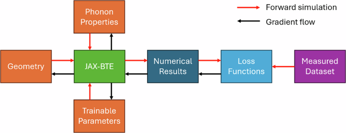
Red arrows indicate the forward simulation flow, while black arrows indicate the gradient flow for inverse modeling.
Specifically, the core solver processes the inputs to perform the forward simulation, yielding outputs such as phonon energy distribution, temperature distributions and heat flux. As depicted in Fig. 10, within the solver, phonon energy densities are stored as a three-dimensional JAX tensor, with indices corresponding to the cell index, band index, and angular index. The solver also utilizes the owner and neighbor lists derived from the geometry to map the phonon energy tensors onto a graph that encodes the topological information of the computational mesh. Using this graph-based representation, the solver efficiently computes the phonon energy densities by solving the discretized algebraic equations in parallel using GPUs. This tensor-based parallelization enables efficient updates of the phonon energy distribution across both structured and unstructured meshes.
Fig. 10: Parallel strategy of the JAX-BTE solver.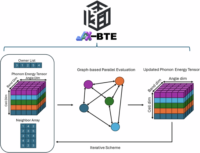
Phonon energy is stored as a 3D JAX tensor. Owner and neighbor lists are used for the construction of graph-based data structure for efficient GPU computing.
For inverse modeling tasks, the JAX-BTE solver facilitates the optimization of unknown or uncertain input parameters by comparing simulated results with experimental measurements. These parameters could include material properties, geometric variables, or heat source intensities. The inverse problem is formulated as an optimization problem, where the objective is to minimize a loss function that quantifies the difference between the simulation outputs (e.g., temperature or heat flux) and the corresponding measured data. Given that JAX-BTE is fully differentiable, the loss function can be expressed as a function of the trainable parameters, and its gradient with respect to these parameters is automatically computed through the AD capabilities of JAX. The differentiability feature in JAX-BTE is enabled by the JAX gradient tracking framework. While AD is used for flux calculations and gradient reconstruction, gradient propagation for implicit components, such as the BiCGSTAB solver, is handled through a discrete adjoint approach. Instead of naively applying AD to iterative steps, which would be computationally inefficient, JAX formulates an additional adjoint equation system and solves it using BiCGSTAB. This hybrid strategy leverages the flexibility of AD for explicit computations while utilizing adjoint methods for iterative solvers, ensuring efficient and scalable gradient tracking even for large-scale phonon BTE simulations. This gradient information enables the use of gradient-based optimization algorithms, such as stochastic gradient descent (SGD), Adam, or L-BFGS, to iteratively update the parameters and minimize the loss. The differentiability of the solver ensures that even complex, high-dimensional parameter spaces can be explored systematically, allowing for accurate recovery of unknown parameters or material properties in a physics-constrained setting.