This section focuses on the specific analysis of the queueing system model proposed in this paper that contains local devices, peer devices, and edge cloud processors, and expands on the four aspects of the task model, local computation model, offloading computation model, and the dynamics of the queueing, and finally gives the optimization problem of this paper.
Task model
In this paper, we consider a computational offloading system with a large number of sensitive tasks arriving randomly in a joint D2D technique with edge cloud, and we investigate the task offloading problem for multiple user devices, multiple peers, and multiple edge clouds. In this system, user devices have a large number of sensitive computational tasks with high latency requirements waiting to be processed on each time slot. We define a time slot to be denoted by t, the duration of each time slot to be \(\tau\) , and set T to be the set of the indexes of the T time slots. The computational task is denoted by \({i} \in \{1,2,\ldots ,N\}\), let N be the set of N tasks, and assume that each task is a whole and cannot be partitioned into task blocks for computation. And the user task must be completed before its deadline \(F_{i}\), otherwise the user program will crash. The computational model architecture for the task is shown in Figure 1. From the system model diagram, we can see that the local device communicates with other peers as well as the edge cloud through a wireless access and offloads the task to the optimal processing location through an offloading link. At the same time, in order to fit the real-world scenarios, both the peer devices and the edge cloud have their own tasks to be processed.
Fig. 1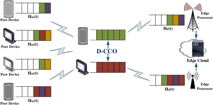
The system model diagram.
When new execution tasks are run on the local device, each task has the option of being processed either on the local device, the peer device, or in the edge cloud server. To this end, we define an offloading decision for each task that identifies where the task is to be computed. The offloading decision is defined as follows:
$$\begin{aligned} \begin{aligned}&{y_{ld}^{i}(t), y_{lm}^{i}(t)} \in \{0,1\}, \\&{y_{ld}^{i}(t)+y_{lm}^{i}(t)} \in \{0,1\}, \end{aligned} \end{aligned}$$
(1)
where \({l}\in \text {L}, {d}\in \text {D}, {m}\in \text {M}\) denote the local device, the peer device, and the edge cloud processor, respectively, \(y_{ld}^{i}(t)=1\) denotes that task i is offloaded to the peer device d for processing, and \(y_{lm}^{i}(t)=1\) denotes that task i is offloaded to the edge cloud m for execution, and when \(y_{ld}^{i}(t), y_{lm}^{i}(t)\) are both 0, it denotes that task i is processed on the local device l. And a task can only be selected to be processed on one processor and cannot be executed on any two or three of the local device, peer device or edge cloud at the same time, so \(y_{ld}^{i}(t), y_{lm}^{i}(t)\) cannot be 1 at the same time.
If the task is migrated to other peer devices in the system or processed on the edge cloud, we assume that the computational latency and energy consumption of the corresponding processor to return the result to the local user device after the computation is completed is negligible. In addition, for the computational task i arriving on the local end device, we define it with a quaternion \({\{D_{i},C_{l}^{i}.C_{ld}^{i},C_{lm}^{i}\}}\), where \(D_{i}\) denotes the size of the amount of data to be processed by the task i itself, and \(C_{l}^{i}\), \(C_{ld}^{i}\), and \(C_{lm}^{i}\) represent the number of CPU cycles to be executed for the computation of the task i on the local device, the other peer devices, and the edge cloud processor, respectively.
Local computational model
In this system, local user devices have different processing rates, while the computing power of the devices themselves is limited. We define the local device to have a large number of sensitive computational tasks arriving in each time slot, and set the transmission power of the local device to be fixed. For local devices in the system, we use the notation \({l} \in \{1,2,\ldots ,L\}\) to denote that L is the set of all local devices in the system. And we use \(f_{l}\) to represent the computing power of the local device, i.e., the number of CPU cycles per second (in GHz/s) that the local user device can execute. According to Dynamic Voltage and Frequency Scaling (DVFS)39, we can also make changes to the computation rate of the local device by adjusting the frequency of this cycle, so that the execution rate of task i on the local device in time slot t is:
$$\begin{aligned} v_{l}^{i}(t)=\eta _{l}^{i}(t)f_{l}, \end{aligned}$$
(2)
where \(0\le \eta _{l}^{i}(t) \le 1\), we define it as the ratio of the actual computing power of the local device to its computing power. Then the computational delay \(t_{l}^{i}\) for task i to process on the local device l is:
$$\begin{aligned} t_{l}^{i}=\frac{C_{l}^{i}}{v_{l}^{i}(t)}. \end{aligned}$$
(3)
In addition, we define \(\rho _{l}^{i}\) to denote the processing power of the device when the task is processed on the local device, then the energy consumption required by the task to computing on the local device can be expressed as:
$$\begin{aligned} e_{l}^{i}=t_{l}^{i}\times \rho _{l}^{i}. \end{aligned}$$
(4)
Offloading computational model
In addition to being able to compute locally, computational tasks on the local device have the option of being offloaded to other processors for processing, and this subsection focuses on the two parts of offloading tasks to peer devices or edge cloud processors specifically. The first is a computational offloading model of offloading tasks to other peers, where there are limited peer resources in the system but plenty of free computational resources. We denote it by \({d} \in \{1,2,\ldots ,D\}\) and the set of peer devices is set to D.
The computational latency of task migration to peers consists of two main phases, the link transmission latency of task offloading to other peers and the processing latency on the peers, with negligible computational latency for the return of computation results to the user locally. In this paper, we define \(f_{d}\) as the computational power of the peer device d, and \(v_{ld}^{i}(t)\) denotes the data transmission rate for offloading task i from the local to the peer device. Using the Shannon formula, the rate is defined as:
$$\begin{aligned} v_{ld}^{i}(t)=\omega log_{2}\bigg (1+\frac{\rho _{ld}^{i}h_{ld}^{i}(t)}{\sigma _{ld}^{i}}\bigg ), \end{aligned}$$
(5)
where \(\omega\) is the transmission bandwidth of the link channel in this queueing system, \(\rho _{ld}^{i}\) represents the transmission power from the local user device offloading task i to the peer device, \(h_{ld}^{i}(t)\) is the channel gain from the local to the peer device channel, and the noise power is denoted by \(\sigma _{ld}^{i}\), which is modeled as obeying additive white Gaussian noise.
In addition, we define \(v_{ld}^{max}(t)\) as the maximum transmission rate of the channel from the user’s local to the peer device. Then, the transmission delay \(t_{ld}^{i}\) computed by task i from local offloading to the peer device is denoted as:
$$\begin{aligned} t_{ld}^{i}=\frac{D_{i}}{v_{ld}^{i}(t)}. \end{aligned}$$
(6)
Meanwhile, the local execution energy consumption for task i to offload to other peers for processing is defined as:
$$\begin{aligned} e_{ld}^{i}=t_{ld}^{i} \times \rho _{ld}^{i}. \end{aligned}$$
(7)
Furthermore, on time slot t, we define the computational power of the peer device to be \(f_{d}\), and then the computational rate of task i on peer device d is:
$$\begin{aligned} v_{d}^{i}(t)=\eta _{d}^{i}(t)f_{d}, \end{aligned}$$
(8)
Where \(\eta _{d}^{i}(t) \in [0,1]\ \) represents the ratio of the actual computing power of the peer device, the processing latency of the task on the peer device can be expressed as:
$$\begin{aligned} t_{d}^{i}=\frac{C_{ld}^{i}}{v_{d}^{i}(t)}. \end{aligned}$$
(9)
And the energy consumption of task processing on the peer device is
$$\begin{aligned} e_{d}^{i}=t_{d}^{i} \times \rho _{d}^{i}, \end{aligned}$$
(10)
Where \(\rho _{d}^{i}\) indicates the processing power of the device when the task is executed on the peer device.
Next, we elaborate the computational offloading model for task offloading to edge cloud processors. Edge cloud processors have outstanding computing power compared to local devices and peers. We denote the edge cloud processor by the symbol \(m \in \{1,2,\ldots ,M\}\) and the set of processors is set to M. Similarly, the total execution latency of task offloading to the edge cloud consists of two components: the transmission latency of the task on the offload link and the processing latency on the edge cloud processor.
First, we define the transmission rate of the task during the offloading of computational communication. And \(v_{lm}^{i}(t)\) is used to denote the transmission rate at which the local user device sends the task to the edge cloud, the formula is as follows:
$$\begin{aligned} v_{lm}^{i}(t)=\omega log_{2}\bigg (1+ \frac{\rho _{lm}^{i}h_{lm}^{i}(t)}{\sigma _{lm}^{i}}\bigg ), \end{aligned}$$
(11)
where \(\rho _{lm}^{i}\) is the transmission power from the task offload to the edge cloud, \(h_{lm}^{i}(t)\) is the channel gain from the local to the edge cloud, and \(\sigma _{lm}^{i}\) represents the noise power of additive Gaussian white noise.
In addition, we further the maximum channel transmission rate from the user’s local to the edge cloud processor, denoted by \(v_{lm}^{max}(t)\). Then the transmission delay of task i offloaded from the local user device to the edge cloud m is defined as:
$$\begin{aligned} t_{lm}^{i}=\frac{D_{i}}{v_{lm}^{i}(t)}. \end{aligned}$$
(12)
Then, the energy consumption generated by the local device during that transmission is:
$$\begin{aligned} e_{lm}^{i}=t_{lm}^{i}\times \rho _{lm}^{i}. \end{aligned}$$
(13)
Meanwhile, we define the computation rate of the task on the edge cloud within the time slot as:
$$\begin{aligned} v_{m}^{i}(t)=\eta _{m}^{i}(t)f_{m}, \end{aligned}$$
(14)
where \(f_{m}\) is the computational power of the edge cloud processor and \(0\le \eta _{m}^{i}(t) \le 1\) is the ratio value of the actual processing power of that edge cloud processor. Then the computational delay of task i on the edge cloud processor m is:
$$\begin{aligned} t_{m}^{i}=\frac{C_{lm}^{i}}{v_{m}^{i}(t)}. \end{aligned}$$
(15)
Queue dynamics
This subsection focuses on the representation of the dynamism of the queue, where we define that the local device, the peer device and the edge processor process one computational task at a time, and the rest of the tasks are stored waiting in their respective queues. We then use an offloading strategy to decide where tasks should be processed to minimize the computational cost while improving the quality of the user’s experience. This queue system model is shown in Figure 1. In the following, we describe the construction of queues in this system in detail.
First, define the queue \(Q_{l}^{i}(t) \in (0,\infty ]\ \) of task i in time slot t on local device l, in which all tasks requiring computation on the local are stored. Also, we define that at each time slot t the local device has a random arrival of a large number of computational tasks that need to be processed, denoted by \(A_{l}^{i}(t)\). We assume that it obeys an independently identically distributed (i.i.d) model and define its mean as \(E[A_{l}^{i}(t)]=\lambda _{l}^{i}\), where \(\lambda _{l}^{i}\) represents the average arrival rate of task i on the local device l. Then the formula for the dynamics of the local device queue in adjacent time intervals is as follows:
$$\begin{aligned} \begin{aligned} Q_{l}^{i}(t+1)&=\bigg [Q_{l}^{i}(t)-v_{l}^{i}(t)-\sum _{d=1}^{D}y_{ld}^{i}(t)v_{ld}^{i}(t) -\sum _{m=1}^{M}y_{lm}^{i}(t)v_{lm}^{i}(t)\bigg ]^{+}+A_{l}^{i}(t), \end{aligned} \end{aligned}$$
(16)
where \([\cdot ]^{+}=max\{\cdot ,0\}\). The first term in the equation represents the current remaining unprocessed computational tasks of the local device, and is non-negative by definition, and is specifically expressed as the length of the task queue at time slot t minus the sum of the amount of locally processable tasks and the tasks offloaded to the other peer devices in the system as well as to the edge cloud processor. Thus the defining construct of this queue is the sum of the remaining unexecuted tasks and newly arriving tasks on the local device.
In addition, we define \(H_{d}^{i}(t)\in [0,\infty )\) as a queue representation of task i on peer device d in time slot t for storing computing tasks arriving on that peer device. And define \(A_{d}^{i}(t)\) obeying i.i.d to denote the random number of arrivals of tasks on peer devices in time slot t, with the average value set to \(E[A_{d}^{i}(t)]=\lambda _{d}^{i}\), where \(\lambda _{d}^{i}\) is the average arrival rate of tasks on peer device d. Then, we represent the definition of the dynamics of the queue on each peer as follows:
$$\begin{aligned} \begin{aligned} H_{d}^{i}(t+1)=\bigg [H_{d}^{i}(t)-v_{d}^{i}(t)\bigg ]^{+}&+\sum _{l=1}^{L}y_{ld}^{i}(t)v_{ld}^{i}(t)+A_{d}^{i}(t). \end{aligned} \end{aligned}$$
(17)
where the first term on the right side of the equation represents the tasks that are still waiting to be processed on the peer device, and the second term represents the tasks that have been offloaded locally to that peer device, so that the sum of the last two terms represents the total new arrivals of tasks on that peer device at time slot t.
Finally, we denote by \(H_{m}^{i}(t)\in [0,\infty )\) the queue of task i on the edge cloud processor m in time slot t. This dynamics formula can be expressed as:
$$\begin{aligned} \begin{aligned} H_{m}^{i}(t+1)=\bigg [H_{m}^{i}(t)-v_{m}^{i}(t)\bigg ]^{+}&+\sum _{l=1}^{L}y_{lm}^{i}(t)v_{lm}^{i}(t)+A_{m}^{i}(t). \end{aligned} \end{aligned}$$
(18)
In the formula, \(A_{m}^{i}(t)\) denotes the random arrivals of tasks on this edge cloud processor in slot t. Assuming that it also obeys i.i.d, and that we define \(\lambda _{m}^{i}\) as the average arrival rate of tasks on the edge cloud processor, the representation of the average value is \(E[A_{m}^{i}(t)]=\lambda _{m}^{i}\). The representation of each item in the formula is the same as above, with the first term being the tasks that have not yet been processed on the edge cloud processor, and the sum of the last two terms represents the total number of new arrivals for that processor at slot t, where the first term is then the tasks that have been offloaded from the local to that processor.
By describing and analyzing the dynamics of the three queues described above, We can find that there is a certain coupling between the above three formulas, i.e., the departure of a task on the local device queue is the arrival of a task on any of the other peer device queues or the edge cloud processor queues in the system. In this system, in order to make it more relevant to real-world scenarios, we defined each queue with newly arriving tasks, which is reflected in the latency of the computed tasks. Therefore, we assume that the item does not affect the coupling relationships described in the text. In addition, we define \(Q_{tot}^{i}(t)\) as the sum of tasks in this system at time slot t and define \(Q_{max}^{i}(t)\) as the maximum number of tasks that can be accepted by the queue, which can be expressed as:
$$\begin{aligned} \begin{aligned} Q_{tot}^{i}(t)&=Q_{l}^{i}(t)+H_{d}^{i}(t)+H_{m}^{i}(t),\\&Q_{tot}^{i}(t)\le Q_{max}^{i}(t). \end{aligned} \end{aligned}$$
(19)
In other words, this formula represents that the total number of computational tasks in time slot t is equal to the sum of the number of tasks of all three, the local device queue, the peer device queue, and the edge cloud processor queue, and that the sum does not exceed the maximum number of tasks that can be received by the queues in the system. If the maximum number of tasks is exceeded, the task may crash and the user experience will be poor. Also, the formula is an equivalent definition of the coupling relationship between queues in the system.
Problem formulation
In this section, we define the optimization problem for this queueing system model. First, we construct a quadratic equation using the Lyapunov optimization technique which combines the three sets of control queues in the system whose main roles are optimized, i.e., local queue \(Q_{l}^{i}(t)\), peer device queue \(H_{d}^{i}(t)\), and edge cloud processor queue \(H_{m}^{i}(t)\). This Lyapunov quadratic function is expressed as:
$$\begin{aligned} \begin{aligned} V(t)=\frac{1}{2}\sum _{l=1}^{L}\sum _{i=1}^{N}[Q_{l}^{i}(t)]^{2}+\frac{1}{2} \sum _{d=1}^{D}\sum _{i=1}^{N}[H_{d}^{i}(t)]^{2}+\frac{1}{2}\sum _{m=1}^{M}\sum _{i=1}^{N}[H_{m}^{i}(t)]^{2}. \end{aligned} \end{aligned}$$
(20)
Based on the definition of queue in the previous subsection, we can conclude that the function is strictly incremental. To ensure that the queues are all bounded and there is no case where a queue has an infinite size, the Lyapunov drift function is defined as:
$$\begin{aligned} \Delta (t)=E[V(t+1)-V(t)|Z(t)], \end{aligned}$$
(21)
where \(Z(t)=\big (Q_{l}^{i}(t);H_{d}^{i}(t);H_{m}^{i}(t)\big )\), denotes the queue vector on the local device, the peer device, and the edge cloud processor in time slot t. From the definition of Lyapunov optimization theory14, by minimizing the drift function, we can optimize the queue backlog on each time slot in this system, and also ensure the stability of this queue system. Therefore, below we give the definition of the optimization problem for this system:
$$\begin{aligned} \begin{aligned}&\max _{y_{ld}^{i}(t),y_{lm}^{i}(t)}\sum _{l=1}^{L}\sum _{i=1}^{N}Q_{l}^{i}(t)\Bigg (v_{l}^{i}(t) +\sum _{d=1}^{D}y_{ld}^{i}(t)v_{ld}^{i}(t)+ \sum _{m=1}^{M}y_{lm}^{i}(t)v_{lm}^{i}(t)-A_{l}^{i}(t)\Bigg )\\&\quad +\sum _{d=1}^{D}\sum _{i=1}^{N}H_{d}^{i}(t)\Bigg (v_{d}^{i}(t) -\sum _{l=1}^{L}y_{ld}^{i}(t)v_{ld}^{i}(t)-A_{d}^{i}(t)\Bigg ) \\&\quad +\sum _{m=1}^{M}\sum _{i=1}^{N}H_{m}^{i}(t)\Bigg (v_{m}^{i}(t) -\sum _{l=1}^{L}y_{lm}^{i}(t)v_{lm}^{i}(t)-A_{m}^{i}(t)\Bigg ) \end{aligned} \end{aligned}$$
(22)
subject to
$$\begin{aligned} \begin{aligned}&(a) \ (1), (19); \\&(b) \ v_{ld}^{i}(t) \le v_{ld}^{max}(t); \\&(b) \ v_{lm}^{i}(t) \le v_{lm}^{max}(t); \\&(c) \ t_{l}^{i}, t_{ld}^{i}+t_{d}^{i}, t_{lm}^{i}+t_{m}^{i}
The four constraints described above denote the conditions to be satisfied for the computational offloading decision of the task, the conditions to be satisfied for the queue in the system, the conditions to be satisfied for the transmission rate of the computational task during the transmission of the task from the user’s local-end device to the peer device and during the transmission of the task from the local-end device to the edge cloud processor, and the conditions of the task completion deadline.
In addition, Eq.(22) is obtained by minimizing the \(\Delta (t)\) in Eq.(21), and by solving this optimization problem, we can minimize the average queue backlog of the tasks on each time slot in the system, improve the computational performance of the user’s tasks, and at the same time achieve the stability of the queues in the system. The concrete proof procedure of this optimization problem is shown in Appendix A. By optimizing this problem, we are able to minimize the computational delay of the task, and based on this, the energy consumption of the task is optimized to minimize the computational cost of the task. To this end, this paper proposes a D2D-assisted collaboration computational offloading strategy (D-CCO) , which comprehensively determines the offloading decisions of the tasks in this system and gets the number of tasks that can be computed at each offloading.