Smart neural network and cognitive computing process for multi task nuclei detection segmentation and classification in breast cancer histopathology images

Cognitive Computing Process (CCP)

CCP allows the model to focus on fine details and critical patterns within the nuclei, leading to more precise learning outcomes. The model is better equipped to accurately diagnose malignancies by honing in on these intricate features. As a result, the CCP significantly improves feature extraction while effectively minimizing the time and computational complexity in the classification process. Unlike traditional methods that depend on images across all magnifications, CCP concentrates explicitly on processing high-magnification (400×) to low-magnification (40×) images. Focusing on these magnification levels, the CCP better analyzed cellular and tissue characteristics, crucial for early breast cancer diagnosis. The CCP enhances the accuracy and effectiveness of the diagnostic process, paving the way for improved outcomes in breast cancer detection.

This proposed work aims to boost the model’s productivity through an efficient and effective learning process by providing high-quality input data. This enhances the model’s ability to diagnose the early stages of breast cancer effectively despite low-magnification images. Figure 5 demonstrates the CCP architecture, and the following approaches are given below.

• Patch generation: Splitting the whole image into patches ensures that the image retains the original features and is compact to our model. To retain the tissue boundary of the nuclei, overlapping patches are generated, and the patches are limited until all the pixels are covered in alternate patches.

• Nuclei segmentation: Segmenting nuclei from input malignant image patches using the advanced Deep U-Net Spatial Attention Model (SAM) accurately identifies and outlines the nuclei within each patch.

• Nucleus density calculation: We meticulously calculated the density of nuclei for the unique malignant patch using micron-per-pixel values, which is crucial for understanding the progression and severity of the malignancy.

• Threshold setting: The patches are classified into low, medium, and high-density categories based on the density of malignant cell nuclei. These clusters are crucial for accurately categorizing the patches according to their characteristics. This method effectively trains our model, leading to a more precise and informed analysis of the early stages of breast cancer.

Fig. 5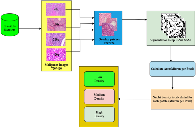Patch generation

The datasets are split based on four specific magnification levels: 40×, 100×, 200×, and 400×. Each class encompasses benign and malignant samples, with every image comprising 700 × 460 pixels. Instead of resizing these images, which leads to a loss of detail, overlap patches measuring 224 × 224 pixels are meticulously extracted at each designated magnification level to regain the boundary of the nuclei and limit the patches until all the pixels are covered, as outlined in Table 3 and shown in Fig. 6.

Fig. 6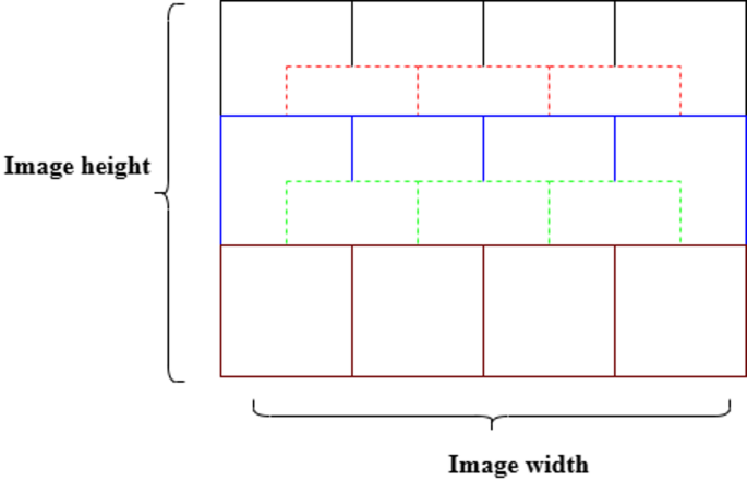

Outline of image patches sized 224 × 224 pixels.

Table 3 Histopathology image samples used in this proposed study.Nuclei segmentation

Detecting overlapped nuclei in histopathology images is challenging due to the hidden features within these images. The U-Net model has become a key framework for medical image segmentation, leading to various adaptations to enhance performance35,36,37,38,39,40. This study employs a Gaussian filter to reduce noise in input patches, resulting in cleaner data for better analysis. Additionally, the deconvolution method is used to remove Hematoxylin-Eosin(H&E) staining, effectively revealing the underlying cellular architecture, and sample stain-removed images are shown in Fig. 7. Our model segments overlapped malignant image patches at different magnifications (40×, 100×, 200×, and 400×) using the Deep U-Net Spatial Attention Model (Deep U-Net SAM), which excels at locating, detecting, and segmenting nuclei. The encoder’s deep feature maps and the decoder’s attention mechanism allow for precise identification and delineation of nuclei in each patch.

Fig. 7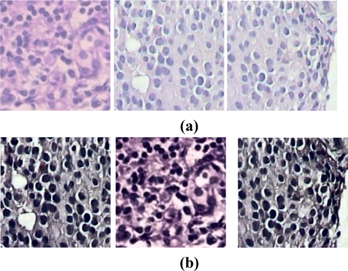

Deconvolution method applied to histopathology images for remove stain (a) Original Image (b) stain-removed image.

Figure 8 demonstrates the proposed Deep U-Net SAM model, which is characterized by a sophisticated architecture that comprises both encoder and decoder sections, working in tandem to process and reconstruct data effectively. Within the encoder, a series of progressive down-sampling operations is meticulously executed, while the decoder employs corresponding up-sampling techniques, both accomplished through the application of convolutional operations. This architecture is built upon a foundation of  × 3 convolutional layers, utilizing a range of filter sizes specifically, 16 × 16, 32 × 32, 64 × 64, 128 × 128, and 256 × 256, ensuring an optimal balance between feature extraction and computational efficiency. Each convolutional layer is fitted with a stride of 2 × 2, which facilitates the gradual reduction of spatial dimensions within the encoder. Moreover, the model incorporates four strategically placed max-pooling layers, each with a pooling size of 3 × 3, further enhancing the dimensionality reduction process while retaining critical features for subsequent stages.

Fig. 8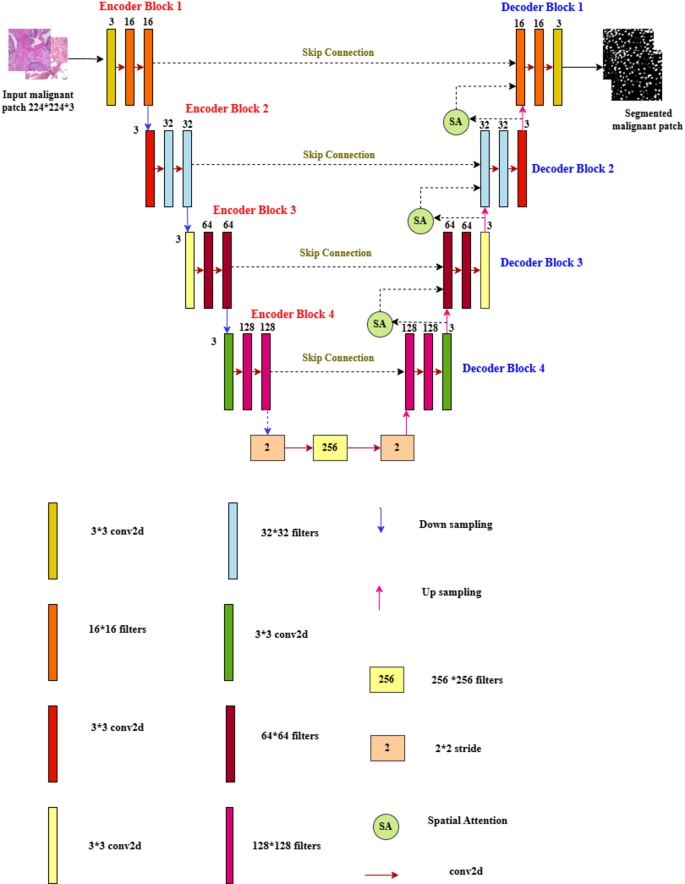

Proposed deep U-Net model with spatial attention mechanism (SAM).

A noteworthy feature of the decoder block is that the layers are integrated with a spatial attention mechanism (SAM), allowing the model to focus on important regions of the data and improving the interpretability and accuracy of the output. To reduce nonlinearity in the model, the Rectified Linear Unit (ReLU) activation function is employed throughout the architecture, ensuring that a wide variety of functions can be learned from the data. Finally, the model culminates in a classification layer that utilizes a sigmoid activation function, effectively converting the output features into probabilities for binary classification tasks. This thoughtful design allows the Deep U-Net SAM model to excel in complex data processing scenarios. Accurate detection of nuclei in histopathology images is essential for successful diagnostic and research applications.

Fig. 9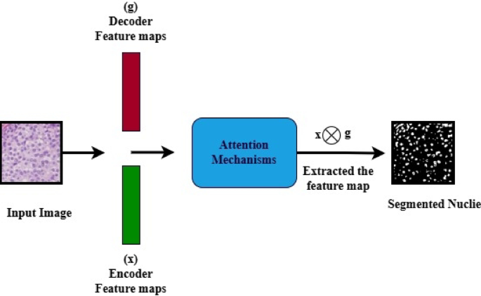

Architecture of the spatial attention mechanisms (SAM).

Figure 9 illustrates Spatial Attention Mechanisms (SAM). In the SAM model, the malignant images are fed into an encoder that extracts spatial features from both the encoder and decoder. The decoder aids in directing the attention mechanisms to focus on the noise and nuclei regions. The attention gates learned to suppress irrelevant background noise and enhanced discriminative features for precision. The attention module multiplies the features from the encoder by attention weights derived from the inputs of both the encoder and decoder, which enhances significant features while diminishing the background. These results improved the efficiency of nuclie segmentation.

The Deep U-Net SAM model is trained over 50 epochs in this approach to ensure it effectively captures the complex features inherent in the input image patches. The specific parameter settings utilized for the Deep U-Net SAM model are meticulously outlined in the accompanying Table 4, providing insight into our methodological choices. Micron-per-pixel measurements are employed to precisely locate the nuclei, significantly improving their spatial identification accuracy. This process involves several well-defined steps, outlined below, to ensure that the model delivers reliable and consistent results in identifying cellular structures within the histopathological images.

Table 4 Parameter settings of the deep U-Net SAM model.Nuclei density calculation

These steps outline the process for calculating nuclei density.

Microscope setup

The BreakHis image datasets were captured using the Olympus BX-50 microscope with a 3.3× relay lens and a Samsung SCC-131AN digital camera. This camera features a 1/3-inch Sony HAD CCD with a pixel size of 6.5 μm × 6.25 μm and a resolution of 752 × 582 pixels, producing 24-bit RGB images. It supports objective lenses with magnifications of 40×, 100×, 200×, and 400×. Original images often have black borders and text annotations, which are cropped for improved quality. Edited images are saved as 700 × 460-pixel PNG files in three-channel RGB format, maintaining visual integrity without artifacts. Pixel size is calculated by dividing the camera’s physical pixel size by the relay and objective lens magnifications.

Microns per pixel calculations

This work uses microns per pixel measurements to analyze cell architecture in histopathology images. Microns are essential in microscopy for determining object sizes and cell structures in whole-slide images, including those in the BreakHis datasets. The micron-per-pixel value represents the physical size of each pixel, calculated from metadata of the datasets referenced in41,42,43. The camera sensor has a consistent pixel size of 6.5 μm across various magnifications (40×, 100×, 200×, and 400×) and lenses (4×, 10×, 20×, and 400×). Magnification depends on the lens, which focuses light for clear imaging, allowing for accurate size representation.

Table 5 shows the micron pixel values for different magnifications using Eq. (1).

$$\:{mpp}_{\:\:\:\:}-\:\frac{pps}{{m}_{\:\:\:\:\:}}{\upmu\:}\text{m}\:$$

(1)

Let, µm, micron meter, \(\:{mpp}_{\:\:\:\:\:}\), micron per pixel, \(\:\:\:\:\:\:\:{pps}_{\:\:\:\:}\), physical pixel size of the lens, \(\:{m}_{\:\:\:\:\:}\) magnification

Table 5 Micron per pixel values at different magnification levels.Nuclei detection

Calculating nuclei density within specific tissue areas is crucial for analyzing cellular composition. This involves measuring microns per pixel along the x and y axes using images at various magnifications (40×, 100×, 200×, and 400×). Higher magnification provides detailed insights into tissue architecture. Nuclei density is determined by the number of nuclei per unit area, converting pixel area into square units. The micron-per-pixel values for the x and y axes are calculated using Eqs. (2) and (3), leading to accurate measurements of nuclei area.

Table 6 illustrates constant values for different BreakHis dataset magnifications. These values remain consistent since the sensor pixel size and magnification factor do not change, ensuring uniform pixel dimensions and quality images.

$$\:{mpp}_{x}\:\:=\:\:\frac{pps}{m\:\:}{\upmu\:}\text{m}$$

(2)

$$\:{mpp}_{y}\:\:\:=\:\:\:\frac{pps}{m\:\:}{\upmu\:}\text{m}$$

(3)

where, \(\:{mpp}_{x}\) is the micron per pixel respective to the x-axis, \(\:{mpp}_{y}\) is the micron per pixel respective to the y-axis.

Table 6 Whole images micron per pixel values with respect to the x and y axis.Estimation of nuclei area

The calculation area of the nuclei is calculated using the following procedures, which are given in detail below.

• Read the height and width of the nuclei in millimeters (mm).

• To accurately locate the nuclei, the height and width of the nuclei are calculated to \(\:{\upmu\:}\text{m}\) using Eqs. (4) and (5).

$$\:{w}_{x}-{w}_{p}\times\:{mpp}_{x}\left({\upmu\:}\text{m}\right)$$

(4)

$$\:{h}_{y}-{h}_{p}\times\:{mpp}_{y}\left({\upmu\:}\text{m}\right)$$

(5)

Equation (6) calculates the nuclei’s area.

$$\:{a}_{n}-{\:\:\:w}_{x}\times\:{h}_{y}\left({{\upmu\:}\text{m}}^{2}\right)$$

(6)

where, \(\:{w}_{x}\) is the Width in micron meter, \(\:{h}_{y}\) is the Height in micron meter, \(\:{w}_{p}\) is the width (mm), \(\:{h}_{p}\) is the height (mm), \(\:{a}_{n}\) is the area of nuclei.

Calculate nuclei density

Table 7 shows nuclei values of unique malignant patches at various magnifications (40×, 100×, 200×, and 400×) along with the corresponding nuclei density. Finally, nuclei density is calculated for unique malignant patches by converting these values using Eqs. (7) and (8).

$$\:{a}_{mms}\:-\:\frac{{a}_{n}}{{10}^{-6}}\:\left({\text{m}\text{m}}^{2}\right)$$

(7)

$$\:{a}_{d}\:-\:\:\frac{n}{{a}_{mms}\:\:}{(\text{m}\text{m}}^{2})$$

(8)

where, \(\:{a}_{mms}\) is the area of nuclei into millimetre square, \(\:{a}_{d}\) is the nuclei density, \(\:n\) is the total number of nuclei present segmentation region.

Table 7 Area and its conversion to square micrometres \(\:\left({{\upmu\:}{m}}^{2}\right)\).Threshold settings

The nuclei density for each patch is calculated to determine its maximum density value. The malignant patches are then categorized based on this maximum nucleus density, using a threshold and a ratio of 30:30:40 for low, medium, and high density across different magnifications (40×, 100×, 200×, and 400×). Table 8 mentioned the total number of malignant density images along with sample images.

Table 8 Samples of malignant nuclei density images (low, medium, and high) with the corresponding patch counts.Dataset split

In this study, the magnifications 40× and 400× are used to highlight the model’s learning process. The malignant patches are classified into three categories based on their nuclei density: LD, MD, and HD. Figure 10 shows the dataset splits methods, and values are represented in Tables 9 and 10. The benign patches of 40× and 400× magnification are split as overlapping patches without measuring nuclei density. Various augmentation methods, including rescaling, zooming, shearing, rotating, and flipping, are applied to patched images using the ImageDataGenerator function with a batch size of 32.

Fig. 10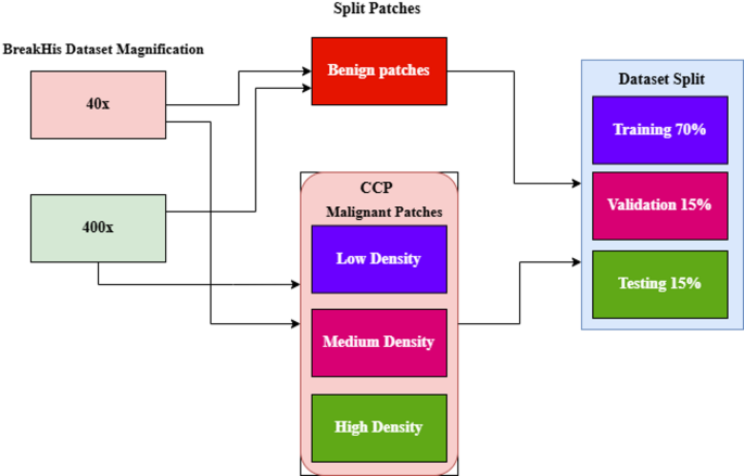

Datasets splitting techniques.

Table 9 Dataset split of benign and malignant density patches at 40× magnification.Table 10 Dataset split of benign and malignant density patches at 400× magnification.SNN models

This methodology aims to enhance the learning rate and improve the efficiency of the learning process. User-defined thresholds calculate the nuclei density in malignant breast tissue histopathology images, classifying it into low, medium, and high levels. The model demonstrates more effective learning on different magnification images to offer a border view of the tissue. Figure 11 illustrates the proposed model architecture.

Fig. 11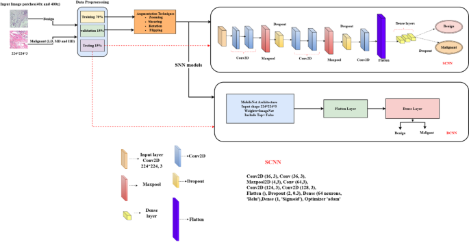

Architecture of the proposed model.

SCNN

To achieve its goals, the CNN model is configured with specialized layers for efficient feature extraction. These layers are crucial for processing complex image data, enabling the model to recognize significant visual patterns that distinguish various nuclei densities. Tailored to detect intricate details, the SCNN architecture enhances classification accuracy, especially with 40x and 400x magnification images. This strategic design is essential for extracting relevant features and ensuring an effective learning process in understanding pathological features in breast tissue samples.

The model includes six 2D convolutional layers with filter sizes of 16, 32, 64, 128, and 256 to extract features from images, using a kernel size of (3, 3). Three 2D max-pooling layers of size (2, 2) reduce feature dimensions. To prevent overfitting, the model incorporates two batch normalization layers and three dropout layers with a retention rate of 30%. Features are flattened into a one-dimensional array and passed to the final classification layer, which consists of two dense layers using the ReLU activation function. However, this approach did not achieve the desired accuracy, prompting the introduction of a new learning strategy model called DCNN.

DCNN

Transfer learning is an effective technique for training the initial layers of deep convolutional neural networks (DCNNs) to recognize image patterns. This research uses pretrained MobileNet networks, trained on the diverse ImageNet dataset with over 20,000 categories, allowing these models to learn rich feature representations that we refine for breast cancer classification44. DCNN model enhances the learning rate using the MobileNet model’s separable convolution architecture for improved feature extraction and model accuracy. The key components include:

• Input layer: Processes incoming data.

• Depthwise convolutional layers: Fourteen layers with filters (32, 64, 128, 256, 512, 1024), a kernel size of (3, 3), and stride (2, 2) for intricate feature extraction.

• Pointwise convolutional layers: Thirteen layers with a kernel size of (1, 1) refine features.

• Batch normalization layers: Twenty-six layers for stabilization and speed.

• ReLU activation layers: Twenty-seven layers for non-linearity and complex pattern capture.

• Zero padding layers: Four layers to maintain spatial dimensions and reduce overfitting.

• Flatten layer: Converts output to one-dimensional for classification.

• Output dense layer: One layer with two neurons for multiclass classification.

DCNN significantly improves learning rate and accuracy over SCNN, making it a robust feature extraction and classification tool.