STAR-RIS enabled covert integration of sensing communication and over-the-air computing with analysis and optimization

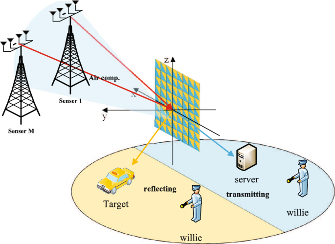
In this section, to evaluate the MSE of AirComp, we consider the joint optimization of the data transmission beamformer \({{\textbf{W}}_{m}}\), radar sensing beamformer \({{\textbf{F}}_{m}}\), data aggregation beamformer \(\textbf{A}\), and the STAR-RIS matrix. Specifically, we aim to optimize the MSE from Equation (8) under the amplitude and phase constraints from Equations (2) and (3), the power constraints from Equation (5), the sensing quality constraints from Equation (22), and the covert communication constraints from Equations (30) and (40).

The optimization framework builds upon the closed-form expressions derived for reliability and security. Specifically, the AirComp MSE, given by \(\mathbb {E}\left[ \left| \textbf{s} – \hat{\textbf{s}}\right| ^2\right]\), quantifies computational reliability and serves as the objective function to be minimized. The security metrics, namely the covert communication rate \(\mathscr {D}\left( \mathbb {P}_0 | \mathbb {P}_1\right) _C \le 2\varepsilon _C^2\) and covert sensing probability \(\tilde{p}\left( \left\{ {{\textbf{F}}_{m}} \right\} ,\textbf{S} \right) \le 2\varepsilon _{S}^{2}\), are derived in closed form (e.g., using the Lambert \(\mathscr {W}\) function for communication covertness), providing explicit constraints that limit signal detectability by eavesdroppers. These expressions are directly integrated into problem (P1), where the MSE defines the optimization goal, and the covertness constraints shape the feasible region for variables \(\textbf{W}_m\), \(\textbf{F}_m\), \(\textbf{A}\), and \(\Theta\). By leveraging these analytical results, we transform the complex joint design into a structured optimization problem, solvable through iterative techniques, thus ensuring that reliability and security are jointly optimized rather than treated in isolation.

$$\begin{aligned}&{\mathbf{(P1)}}\mathop {\min }\limits _{{\varvec{\Theta }},{\textbf{A}},\left\{ {{{\textbf{W}}_m}} \right\} ,\left\{ {{{\textbf{F}}_m}} \right\} } \sum \limits _{m = 1}^M {{\mathop {\textrm{tr}}\nolimits } } \left( {\left( {{{\textbf{A}}^H}{{\textbf{H}}_m}{{\textbf{W}}_m} – {\textbf{I}}} \right) {{\left( {{{\textbf{A}}^H}{{\textbf{H}}_m}{{\textbf{W}}_m} – {\textbf{I}}} \right) }^H}} \right) \\&+ \sum \limits _{m = 1}^M {{\mathop {{\textrm{tr}}}\nolimits } } \left( {{{\textbf{A}}^H}{{\textbf{R}}_m}{{\textbf{F}}_m}{\textbf{F}}_m^H{\textbf{R}}_m^H{\textbf{A}}} \right) + \sigma _c^2{\mathop {{\textrm{tr}}}\nolimits } \left( {{\textbf{A}}{{\textbf{A}}^H}} \right) \end{aligned}$$

(41)

$$\begin{aligned}&s.t.\quad {\mathop {{\textrm{tr}}}\nolimits } \left( {{{\left( {{{\textbf{F}}_m}{\textbf{F}}_m^H} \right) }^{ – 1}}} \right) \le \frac{{T{\eta _m}}}{{{N_{rr}}\sigma _r^2}},\forall m, \end{aligned}$$

(41a)

$$\begin{aligned}&{\mathop {{\textrm{tr}}}\nolimits } \left( {{{\textbf{W}}_m}{{\textbf{W}}_m}^H} \right) + {\mathop {\textrm{tr}}\nolimits } \left( {{{\textbf{F}}_m}{{\textbf{F}}_m}^H} \right) \le P,\forall m., \end{aligned}$$

(41b)

$$\begin{aligned}&{\mathop {\textrm{CRB}}\nolimits } (\tilde{\varphi }) \le \Upsilon , \end{aligned}$$

(41c)

$$\begin{aligned}&\mathscr {D}\left( \mathbb {P}_{0} \Vert \mathbb {P}_{1}\right) _{C} \le 2 \epsilon _{C}^{2}, \end{aligned}$$

(41d)

$$\begin{aligned}&\tilde{p}\left( \left\{ \textbf{F}_{m}\right\} , \textbf{S}\right) \le 2 \epsilon _{S} ^{2}. \end{aligned}$$

(41e)

The optimization problem (P1) involves multiple constraints, including the CRB threshold \(\operatorname {CRB}(\hat{\varphi }) \le \Upsilon\), covert communication constraint \(\mathscr {D}\left( \mathbb {P}_0 | \mathbb {P}_1\right) _C \le 2\varepsilon _C^2\), and covert sensing constraint \(\tilde{p}\left( \left\{ \textbf{F}_{m}\right\} , \textbf{S}\right) \le 2 \epsilon _{S} ^{2}\). These constraints are coupled through the beamforming vectors \(\textbf{W}_m\), \(\textbf{F}_m\), \(\textbf{A}\), and the STAR-RIS matrix \(\Theta\). For instance, a stringent CRB threshold requires higher power allocation to \(\textbf{F}_m\) to enhance sensing SNR, which may increase the sensing eavesdropping probability \(\tilde{p}\left( \left\{ \textbf{F}_{m}\right\} , \textbf{S}\right)\), potentially violating the covert sensing constraint. Similarly, the covert communication constraint limits the power and direction of \(\textbf{W}_m\), which could degrade the AirComp MSE due to reduced signal strength at the server. Moreover, the shared power budget P introduces a trade-off between sensing (via \(\textbf{F}_m\)) and communication (via \(\textbf{W}_m\)), further complicating the optimization. These interactions suggest that overly strict constraints (e.g., very low \(\Upsilon\), \(\varepsilon _C\), or \(\varepsilon _S\)) might shrink the feasible region, potentially rendering the problem infeasible. To address this, our proposed smoothed exact penalty algorithm with CCCP iteratively adjusts the variables to balance these trade-offs, ensuring a feasible local optimum within practical parameter ranges.

Due to the coupling relationships between \(\varvec{\Theta }\), \(\textbf{A}\), \({{\textbf{W}}_{m}}\) and \({{\textbf{F}}_{m}}\), this problem lacks convexity. To ad-dress this issue, we propose an optimal design for the transmission beamforming.

Given the objective of minimizing AirComp MSE, it can be observed that both \(\sum \limits _{m=1}^{M}{\operatorname {tr}}\left( \left( {{\textbf{A}}^{H}}{{\textbf{H}}_{m}}{{\textbf{W}}_{m}}-\textbf{I} \right) {{\left( {{\textbf{A}}^{H}}{{\textbf{H}}_{m}}{{\textbf{W}}_{m}}-\textbf{I} \right) }^{H}} \right)\) and \(\sigma _{c}^{2}\operatorname {tr}\left( \textbf{A}{{\textbf{A}}^{H}} \right)\) are positive. Therefore, for any given data beamforming, the following inequality always holds:

$$\begin{aligned} \sum \limits _{m = 1}^M {{\mathop {{\textrm{tr}}}\nolimits } } \left( {\left( {{{\textbf{A}}^H}{{\textbf{H}}_m}{{\textbf{W}}_m} – {\textbf{I}}} \right) {{\left( {{{\textbf{A}}^H}{{\textbf{H}}_m}{{\textbf{W}}_m} – {\textbf{I}}} \right) }^H}} \right) + \sigma _c^2{\mathop {{\textrm{tr}}}\nolimits } \left( {{\textbf{A}}{{\textbf{A}}^H}} \right) \ge \sigma _c^2{\mathop {{\textrm{tr}}}\nolimits } \left( {{\textbf{A}}{{\textbf{A}}^H}} \right) \end{aligned}$$

(42)

Thus, it is straightforward to demonstrate that for a given data aggregation beam-former \(\textbf{A}\), the zero-forcing transmission beamformer at the sensor minimizes the computation error, given by \({{\textbf{W}}_m} = {\left( {{\textbf{H}}_m^H{\textbf{A}}{{\textbf{A}}^H}{{\textbf{H}}_m}} \right) ^{ – 1}}{\textbf{H}}_m^H{\textbf{A}},\forall m\). The corresponding problem can therefore be formulated as:

$$\begin{aligned}&{\mathbf{(P2)}}\mathop {\min }\limits _{{\varvec{\Theta }},{\textbf{A}},\left\{ {{{\textbf{W}}_m}} \right\} ,\left\{ {{{\textbf{F}}_m}} \right\} } \sum \limits _{m = 1}^M {{\mathop {\textrm{tr}}\nolimits } } \left( {\left( {{{\textbf{A}}^H}{{\textbf{H}}_m}{{\textbf{W}}_m} – {\textbf{I}}} \right) {{\left( {{{\textbf{A}}^H}{{\textbf{H}}_m}{{\textbf{W}}_m} – {\textbf{I}}} \right) }^H}} \right) \\&+ \sum \limits _{m = 1}^M {{\mathop {\textrm{tr}}\nolimits } } \left( {{{\textbf{A}}^H}{{\textbf{R}}_m}{{\textbf{F}}_m}{\textbf{F}}_m^H{\textbf{R}}_m^H{\textbf{A}}} \right) + \sigma _c^2{\mathop {\textrm{tr}}\nolimits } \left( {{\textbf{A}}{{\textbf{A}}^H}} \right) \end{aligned}$$

(43)

$$\begin{aligned}&s.t.\quad {\mathop {\textrm{tr}}\nolimits } \left( {{{\left( {{{\textbf{F}}_m}{\textbf{F}}_m^H} \right) }^{ – 1}}} \right) \le \frac{{T{\eta _m}}}{{{N_{rr}}\sigma _r^2}},\forall m, \end{aligned}$$

(43a)

$$\begin{aligned}&{\mathop {\textrm{tr}}\nolimits } \left( {{{\left( {{\textbf{H}}_m^H{\textbf{A}}{{\textbf{A}}^H}{{\textbf{H}}_m}} \right) }^{ – 1}}} \right) + {\mathop {\textrm{tr}}\nolimits } \left( {{{\textbf{F}}_m}{{\textbf{F}}_m}^H} \right) \le P,\forall m, \end{aligned}$$

(43b)

$$\begin{aligned}&{\mathop {\textrm{CRB}}\nolimits } (\tilde{\varphi }) \le \Upsilon , \end{aligned}$$

(43c)

$$\begin{aligned}&\mathscr {D}\left( \mathbb {P}_{0} \Vert \mathbb {P}_{1}\right) _{C} \le 2 \epsilon _{C}^{2} \end{aligned}$$

(43d)

$$\begin{aligned}&\tilde{p}\left( \left\{ \textbf{F}_{m}\right\} , \textbf{S}\right) \le 2 \epsilon _{S} ^{2} \end{aligned}$$

(43e)

Due to the coupling of variables \(\varvec{\Theta }\), \(\textbf{A}\), and \({{\textbf{F}}_{m}}\) in the objective function, problem (P2)(P2)(P2) is non-convex. Following the standard methods in MIMO beamforming literature41,42,43, the radar sensing beamformer \({{\textbf{F}}_{m}}\) is constrained to be an orthogonal matrix. Mathematically, this can be expressed as \({{\textbf{F}}_{m}}=\sqrt{{\textrm{B}_{m}}}{{\textbf{D}}_{m}}\), where \({{\textbf{D}}_{m}}\) is a unitary matrix, hence \({{\textbf{D}}_{m}}\textbf{D}_{m}^{H}=\textbf{I}\), and \(\sqrt{{\textrm{B}_{m}}}\) is a positive scaling factor. The corresponding problem can be represented as:

$$\begin{aligned}&{\mathbf{(P3)}}\mathop {\min }\limits _{{\varvec{\Theta }},{\textbf{A}},\{ \mathrm{B_m}\} } \sum \limits _{m = 1}^M {\mathrm{B_m}} {\mathop {\textrm{tr}}\nolimits } \left( {{\textbf{R}}_m^H{\textbf{A}}{{\textbf{A}}^H}{{\textbf{R}}_m}} \right) + \sigma _c^2{\mathop {\textrm{tr}}\nolimits } \left( {{\textbf{A}}{{\textbf{A}}^H}} \right) \end{aligned}$$

(44)

$$\begin{aligned}&{\textrm{s}}{\mathrm{.t}}{\mathrm{. }}\quad \frac{{{N_{tx}}}}{{{\textrm{B}_m}}} \le \frac{{T{\eta _m}}}{{{N_{rx}}\sigma _r^2}},\forall m{\textrm{,}} \end{aligned}$$

(44a)

$$\begin{aligned}&{\mathop {\textrm{tr}}\nolimits } \left( {{{\left( {{\textbf{H}}_m^H{\textbf{A}}{{\textbf{A}}^H}{{\textbf{H}}_m}} \right) }^{ – 1}}} \right) + {\textrm{B}_m} \le P,\forall m, \end{aligned}$$

(44b)

$$\begin{aligned}&{\mathop {\textrm{CRB}}\nolimits } (\tilde{\varphi }) \le \Upsilon , \end{aligned}$$

(44c)

$$\begin{aligned}&\mathscr {D}\left( \mathbb {P}_{0} \Vert \mathbb {P}_{1}\right) _{C} \le 2 \epsilon _{C}^{2} \end{aligned}$$

(44d)

$$\begin{aligned}&\tilde{p}\left( \left\{ \textbf{F}_{m}\right\} , \textbf{S}\right) \le 2 \epsilon _{S} ^{2} \end{aligned}$$

(44e)

It can be observed that an increase in \({\textrm{B}_{m}}\) leads to an increase in MSE. Therefore, when using minimal \(\mathrm B_{m}^{*}\) for all \({\textrm{B}_{m}}\), the MSE is minimized, given by \(\alpha _m^* = \frac{{{N_{rt}}{N_{rr}}\sigma _r^2}}{{T{\eta _m}}},\forall m\). By introducing \(\mathbf {\hat{A}}=\textbf{A}{{\textbf{A}}^{H}}\) and applying Semidefinite Relaxation (SDR), the problem can be represented as:

$$\begin{aligned}&{\mathbf{(P4)}}\mathop {\min }\limits _{{\varvec{\Theta }},{\mathbf{{\hat{A}}}}} \sum \limits _{m = 1}^M {\frac{{{N_{tx}}{N_{rx}}\sigma _r^2}}{{T{\eta _m}}}} {\mathop {\textrm{tr}}\nolimits } \left( {{\textbf{R}}_m^H\widehat{\textbf{A}}{{\textbf{R}}_m}} \right) + \sigma _c^2{\mathop {\textrm{tr}}\nolimits } (\widehat{\textbf{A}}) \end{aligned}$$

(45)

$$\begin{aligned}&{\textrm{s}}{\mathrm{.t}}{\mathrm{. }}\quad {\mathop {\textrm{tr}}\nolimits } \left( {{{\left( {{\textbf{H}}_m^H\widehat{\textbf{A}}{{\textbf{H}}_m}} \right) }^{ – 1}}} \right) + \frac{{{N_{rt}}{N_{tt}}\sigma _r^2}}{{T{\eta _m}}} \le P,\forall m, \end{aligned}$$

(45a)

$$\begin{aligned} \widehat{\textbf{A}} \ge 0, \end{aligned}$$

(45b)

$$\begin{aligned}&{\mathop {\textrm{CRB}}\nolimits } (\tilde{\varphi }) \le \Upsilon , \end{aligned}$$

(45c)

$$\begin{aligned}&\mathscr {D}\left( \mathbb {P}_{0} \Vert \mathbb {P}_{1}\right) _{C} \le 2 \epsilon _{C}^{2}, \end{aligned}$$

(45d)

$$\begin{aligned}&\tilde{p}\left( \left\{ \textbf{F}_{m}\right\} , \textbf{S}\right) \le 2 \epsilon _{S} ^{2}. \end{aligned}$$

(45e)

Next, we address the covert communication constraint \({\mathscr {D}}{\left( {{\mathbb {P}_0}{\mathbb {P}_1}} \right) _C} = M\left[ {\ln \left( {\frac{{{{(p_m^C)}^2}{{\left| {{{\textbf{H}}_{m,{W_C}}}} \right| }^2} + \sigma _w^2}}{{\sigma _w^2}}} \right) } \right. \left. { + \frac{{\sigma _w^2}}{{{{(p_m^C)}^2}{{\left| {{{\textbf{H}}_{m,{W_C}}}} \right| }^2} + \sigma _w^2}} – 1} \right]\), and introduce a new variable, denoted as \(x\triangleq \frac{{{\sigma }_{1}}}{{{\sigma }_{0}}}=\frac{{{(p_{m}^{C})}^{2}}{{\left| {{\textbf{H}}_{m,{{W}_{C}}}} \right| }^{2}}+\sigma _{w}^{2}}{\sigma _{w}^{2}}\). Therefore, the constraint \({\mathscr {D}}{{\left( {{\mathbb {P}}_{0}}\Vert {{\mathbb {P}}_{1}} \right) }_{C}}\le 2{{{\epsilon }}_{C}}^{2}\) can be reformulated as:

$$\begin{aligned} f(x) \triangleq \ln x+\frac{1}{x} \le 1+2 \epsilon _{C} ^{2} \end{aligned}$$

(46)

By introducing \(x_1\) and \(x_2\) as the two roots of \(f(x) = 1 + 2\varepsilon _C^2\), where \(f(x) = \ln x + \frac{1}{x}\) is an increasing function over \(\left[ x_1, x_2\right]\), we transform \(\mathscr {D}\left( \mathbb {P}_0 | \mathbb {P}1\right) C \le 2\varepsilon _C^2\) into \(x_1 \le x \le x_2\). Here, \(x_1 =\) \(\exp \left( \mathscr {W}_{-1}\left( -\exp \left( -\left( 1 + 2\varepsilon _C^2\right) \right) \right) + 1 + 2\varepsilon _C^2\right)\) and \(x_2 =\) \(\exp \left( \mathscr {W}_0\left( -\exp \left( -\left( 1 + 2\varepsilon _C^2\right) \right) \right) + 1 + 2\varepsilon _C^2\right)\), with \(\mathscr {W}_{-1}\) and \(\mathscr {W}_0\) denoting the −1 and 0 branches of the Lambert \(\mathscr {W}\) function, respectively. The argument of \(\mathscr {W}{-1}\), \(z = -\exp \left( -\left( 1 + 2\varepsilon _C^2\right) \right)\), must satisfy \(-\frac{1}{e} \le z for \(\mathscr {W}{-1}\) to be defined. Since \(\varepsilon _C^2 \ge 0\) and typically small in covert systems (e.g., \(0 ), we have \(-\exp (-1) \le z , ensuring \(z \ge -\frac{1}{e}\) when \(\varepsilon _C^2 \le \frac{\ln 2}{2}\). For consistency, we assume \(\varepsilon _C^2 \le \frac{\ln 2}{2}\) in this work, which aligns with practical covertness requirements and keeps z within the valid domain. Given that \(x=1+\frac{{{(p_{m}^{C})}^{2}}{{\left| {{\textbf{H}}_{m,{{W}_{C}}}} \right| }^{2}}}{\sigma _{w}^{2}}>1\), we obtain \(0.Thus, problem (P4) can be rewritten as:

$$\begin{aligned}&{\mathbf{(P5)}}\mathop {\min }\limits _{{\varvec{\Theta }},{\mathbf{{\hat{A}}}}} \sum \limits _{m = 1}^M {\frac{{{N_{tx}}{N_{rx}}\sigma _r^2}}{{T{\eta _m}}}} {\mathop {\textrm{tr}}\nolimits } \left( {{\textbf{R}}_m^H\widehat{\textbf{A}}{{\textbf{R}}_m}} \right) + \sigma _c^2{\mathop {\textrm{tr}}\nolimits } (\widehat{\textbf{A}}) \end{aligned}$$

(47)

$$\begin{aligned}&{\textrm{s}}{\mathrm{.t}}{\mathrm{. }}\quad {\mathop {\textrm{tr}}\nolimits } \left( {{{\left( {{\textbf{H}}_m^H\widehat{\textbf{A}}{{\textbf{H}}_m}} \right) }^{ – 1}}} \right) + \frac{{{N_{rt}}{N_{tt}}\sigma _r^2}}{{T{\eta _m}}} \le P,\forall m, \end{aligned}$$

(47a)

$$\begin{aligned}&\widehat{\textbf{A}} \ge 0, \end{aligned}$$

(47b)

$$\begin{aligned}&{\mathop {\textrm{CRB}}\nolimits } (\tilde{\varphi }) \le \Upsilon , \end{aligned}$$

(47c)

$$\begin{aligned}&0

(47d)

$$\begin{aligned} \tilde{p}\left( \left\{ \textbf{F}_{m}\right\} , \textbf{S}\right) \le 2 \epsilon _{S} ^{2}. \end{aligned}$$

(47e)

Given \(\varvec{\Theta }\), the optimization in problem (47) can be reduced to an unconstrained optimization problem, denoted as \(\underset{\widehat{\textbf{A}}}{\mathop {\min }}\,\text {MS}{{\text {E}}_{\widehat{\textbf{A}}}}\). Based on the principles of optimal Minimum Mean Squared Error (MMSE) receiver design, the optimal solution for \(\widehat{\textbf{A}}\) is expressed as \({\textbf{U}}_a^o = {\left( {{\textbf{A}} + \sigma _c^2{\mathop {\textrm{tr}}\nolimits } (\widehat{\textbf{A}})} \right) ^{ – 1}}{\textbf{C}}\). where, \({\textbf{A}} = \sum \limits _{m = 1}^M {{\textbf{R}}_m^H{{\textbf{R}}_m}}\), \({\textbf{C}} = \sum \limits _{m = 1}^M {{{\textbf{R}}_m}}\). Additionally, we set \(d = \sum \limits _{m = 1}^M {{{(p_m^C)}^2}{{\left| {{{\textbf{H}}_{m,{W_C}}}} \right| }^2}}\). The constraint (52 d) can be rewritten \(d \le \left( {{x_2} – 1} \right) \left( {\sigma _w^2} \right)\), Substituting Equations \({\textbf{U}}_a^o\) and d into Equation \(0, problem (P5) can be formulated as:

$$\begin{aligned}&{\mathbf{(P6)}}\mathop {\min }\limits _{{\varvec{\Theta }},{\mathbf{{\hat{A}}}}} \sum \limits _{m = 1}^M {\frac{{{N_{tx}}{N_{rx}}\sigma _r^2}}{{T{\eta _m}}}} {\mathop {\textrm{tr}}\nolimits } \left( {{\textbf{R}}_m^H\widehat{\textbf{A}}{{\textbf{R}}_m}} \right) + \sigma _c^2{\mathop {\textrm{tr}}\nolimits } (\widehat{\textbf{A}}) \end{aligned}$$

(48)

$$\begin{aligned}&{\textrm{s}}{\mathrm{.t}}{\mathrm{. }}\quad {\mathop {\textrm{tr}}\nolimits } \left( {{{\left( {{\textbf{H}}_m^H\widehat{\textbf{A}}{{\textbf{H}}_m}} \right) }^{ – 1}}} \right) + \frac{{{N_{rt}}{N_{tt}}\sigma _r^2}}{{T{\eta _m}}} \le P,\forall m, \end{aligned}$$

(48a)

$$\begin{aligned}&\widehat{\textbf{A}} \ge 0, \end{aligned}$$

(48b)

$$\begin{aligned}&{\mathop {\textrm{CRB}}\nolimits } (\tilde{\varphi }) \le \Upsilon , \end{aligned}$$

(48c)

$$\begin{aligned}&{\textbf{A}} = \sum \limits _{m = 1}^M {{\textbf{R}}_m^H{{\textbf{R}}_m}} , \end{aligned}$$

(48d)

$$\begin{aligned}&{\textbf{C}} = \sum \limits _{m = 1}^M {{{\textbf{R}}_m}}, \end{aligned}$$

(48e)

$$\begin{aligned}&d = \sum \limits _{m = 1}^M {{{(p_m^C)}^2}{{\left| {{{\textbf{H}}_{m,{W_C}}}} \right| }^2}}, \end{aligned}$$

(48f)

$$\begin{aligned}&\tilde{p}\left( \left\{ \textbf{F}_{m}\right\} , \textbf{S}\right) \le 2 \epsilon _{S} ^{2}. \end{aligned}$$

(48g)

where \(\Gamma =\frac{{{N}_{tx}}{{N}_{rx}}\sigma _{r}^{2}}{T{{\eta }_{m}}}\), K represent the number of sensors, and \({{N}_{s}}\) represents the number of antennas equipped on the sensors. Since the objective function (48) and the equality constraints (48 d), (48e), (48f) are non-convex, problem (P5) remains non-convex. Therefore, finding a global optimal solution to optimization problem (58) is challenging. We can transform (48 d), (48e), and (48f) into appropriate convex forms, allowing us to obtain a local optimal solution using the constrained concave-convex procedure (CCCP).

Assuming \(\textbf{Y}\succ \textbf{0}\), \(\varvec{\Omega }={{\textbf{X}}^{H}}{{\textbf{Y}}^{-1}}\textbf{X}\) is equivalent to:

$$\begin{aligned} \left[ \begin{array}{cc} \varvec{\Omega } & \textbf{X}^{H} \\ \textbf{X} & \textbf{Y} \end{array}\right] \succeq \textbf{0} \end{aligned}$$

(49)

and \({\mathop {\textrm{tr}}\nolimits } \left( {{\varvec{\Omega }} – {{\textbf{X}}^H}{{\textbf{Y}}^{ – 1}}{\textbf{X}}} \right) \le 0\).

Let us define auxiliary variables \(\textbf{T}\) and \(\textbf{s}\) as:

$$\begin{aligned} {\textbf{T}} = \left[ {{{\textbf{R}}_1}, \cdots ,{{\textbf{R}}_M}} \right] \end{aligned}$$

(50)

$$\begin{aligned} {\textbf{s}} = \left[ {{{(p_1^C)}^2}{{\left| {{{\textbf{H}}_{1,{W_C}}}} \right| }^2}, \cdots ,{{(p_K^C)}^2}{{\left| {{{\textbf{H}}_{K,{W_C}}}} \right| }^2}} \right] \end{aligned}$$

(51)

The equality constraints (48 d) and (48f) can be equivalently represented as:

$$\begin{aligned} & \left[ \begin{array}{cc} \textbf{A} & \textbf{T} \\ \textbf{T}^{H} & \textbf{I} \end{array}\right] \succeq \textbf{0} \end{aligned}$$

(52)

$$\begin{aligned} & {\mathop {\textrm{tr}}\nolimits } \left( {{{\textbf{A}}_a} – {\textbf{T}}{{\textbf{T}}^H}} \right) \le 0 \end{aligned}$$

(53)

$$\begin{aligned} & \left[ \begin{array}{cc} d & \textbf{s} \\ \textbf{s}^{H} & \textbf{I} \end{array}\right] \succeq \textbf{0} \end{aligned}$$

(54)

$$\begin{aligned} & {\mathop {\textrm{tr}}\nolimits } \left( {d – {\textbf{S}}{{\textbf{S}}^H}} \right) \le 0 \end{aligned}$$

(55)

Thus, problem (P6) can be reformulated as:

$$\begin{aligned} \mathop {\min }\limits _\Xi K{N_s} – {\mathop {\textrm{tr}}\nolimits } \left( {{{\textbf{C}}^H}{{\left( {{\textbf{A}} + {\textbf{B}} + \sigma _a^2{{\textbf{I}}_{{N_r}}}} \right) }^{ – 1}}{\textbf{C}}} \right) \nonumber \\ {\textrm{s}}{\mathrm{.t}}{\mathrm{. (48a),(48b),(48c), (48e),(48f),(48g),(50) – (55)}} \end{aligned}$$

(56)

where \(\Xi =\left\{ {{\textbf{W}}_{k}},\textbf{V},\textbf{T},\textbf{s},\textbf{A},\textbf{B},\textbf{C},d,e \right\}\) in problem (56), constraints (52) and 67 are linear matrix inequalities. Constraints (58) and (48f) are linear. However, the objective function (56), constraints (53), and (55) remain non-convex and exhibit a Difference of Convex (DC) structure. To solve problem (41), we first transform problem (41) into a DC programming problem and then use a penalty-based algorithm to obtain a local optimal solution.

Thus, define \(\Upsilon \triangleq \{\textbf{A},\textbf{C}\}\), \(\Gamma \triangleq \{\textbf{A},d\}\), \(\Psi \triangleq \{\textbf{T},\textbf{s}\}\) along with the function:

$$\begin{aligned} f(\Upsilon )= & {\mathop {\textrm{tr}}\nolimits } \left( {{{\textbf{C}}^H}{{\left( {{\textbf{A}} + \sigma _a^2{{\textbf{I}}_{{N_r}}}} \right) }^{ – 1}}{\textbf{C}}} \right) \end{aligned}$$

(57)

$$\begin{aligned} f(\Gamma )= & {\mathop {\textrm{tr}}\nolimits } ({\textbf{A}} + d) \end{aligned}$$

(58)

$$\begin{aligned} f(\Psi )= & {\mathop {\textrm{tr}}\nolimits } \left( {{\textbf{T}}{{\textbf{T}}^H} + {\textbf{s}}{{\textbf{s}}^H}} \right) \end{aligned}$$

(59)

Using a penalty-based exact algorithm, we can reformulate problem (69) as:

$$\begin{aligned} \mathop {\min }\limits _{\Xi \in \Theta } K{N_s} – f(\Upsilon ) + p(f(\Gamma ) – f(\Psi )) \end{aligned}$$

(60)

\(\text{where}:\,\buildrel \Delta \over = \{ \Xi \mid {\mathrm{(48a),(48b),(48c), (48e),(48f),(48g),(50) – (55),(54)}}\}\), p represents the penalty factor. We can then solve problem (73) using a CCCP-based algorithm. The first-order Taylor series expansions of \(f(\Upsilon )\) and \(f(\Psi )\) around points \(\bar{\Upsilon }\) and \(\bar{\Psi }\) are given by:

$$\begin{aligned} & \begin{array}{l} f(\Upsilon ;\bar{\Upsilon }) = – {\mathop {\textrm{tr}}\nolimits } \left( {{{\overline{\textbf{C}} }^H}{{\left( {\overline{\textbf{A}} + \sigma _a^2{{\textbf{I}}_{{N_r}}}} \right) }^{ – 1}}\overline{\textbf{C}} } \right) + 2\mathbb {R}\left\{ {{\mathop {\textrm{tr}}\nolimits } \left( {{{\overline{\textbf{C}} }^H}{{\left( {\overline{\textbf{A}} + \sigma _a^2{{\textbf{I}}_{{N_r}}}} \right) }^{ – 1}}{\textbf{C}}} \right) } \right\} \\ -\mathbb {R} \left\{ {tr \left( {{{\overline{\textbf{C}} }^H}{{\left( {\overline{\textbf{A}} + \sigma _a^2{{\textbf{I}}_{{N_r}}}} \right) }^{ – 1}}({\textbf{A}} – \overline{\textbf{A}} )} \right. } \right. \left. {\left. { \cdot {{\left( {\overline{\textbf{A}} + \sigma _a^2{{\textbf{I}}_{{N_r}}}} \right) }^{ – 1}}\overline{\textbf{C}} } \right) } \right\} \end{array} \end{aligned}$$

(61)

$$\begin{aligned} & \begin{array}{l} f(\Psi ;\bar{\Psi }) = – {\mathop {\textrm{tr}}\nolimits } \left( {\overline{\textbf{T}} {{\overline{\textbf{T}} }^H} + \overline{\textbf{s}} {{\overline{\textbf{s}} }^H}} \right) + 2\mathbb {R}\left\{ {{{\textrm{tr}}}\left( {{\textbf{T}}{{\overline{\textbf{T}} }^H} + {\textbf{s}}{{\overline{\textbf{s}} }^H}} \right) } \right\} \end{array} \end{aligned}$$

(62)

Assuming \(\left( {{\Upsilon }^{(m)}},{{\Psi }^{(m)}} \right)\) is optimal in the m-th iteration, problem (60) can be formulated as:

$$\begin{aligned} \mathop {\min }\limits _{\Xi \in \Theta } K{N_s} – f\left( {\Upsilon ;{\Upsilon ^{(m)}}} \right) + p\left( {f(\Gamma ) – f\left( {\Psi ;{\Psi ^{(m)}}} \right) } \right) \end{aligned}$$

(63)

where the optimal \(\textbf{A}\),\(\textbf{C}\),\(\textbf{d}\),\(\textbf{e}\),\(\textbf{s}\),\({{\textbf{W}}_{k}}\),\(\textbf{T}\),\(\textbf{V}\) in the m-th iteration are denoted as \({{\textbf{A}}^{\left( m \right) }}\),\({{\textbf{B}}^{\left( m \right) }}\),\({{\textbf{C}}^{\left( m \right) }}\),\({{\textbf{d}}^{\left( m \right) }}\),\({{\textbf{e}}^{\left( m \right) }}\),\({{\textbf{s}}^{\left( m \right) }}\),\(\textbf{W}_{k}^{\left( m \right) }\),\({{\textbf{T}}^{\left( m \right) }}\),\({{\textbf{V}}^{\left( m \right) }}\)

To address the optimization problem, we propose a CCCP-based optimization algorithm, with its detailed steps outlined in Table 1. The algorithm iteratively updates the variables \({{\textbf{A}}^{\left( m \right) }}\),\({{\textbf{B}}^{\left( m \right) }}\),\({{\textbf{C}}^{\left( m \right) }}\),\({{\textbf{d}}^{\left( m \right) }}\),\({{\textbf{e}}^{\left( m \right) }}\),\({{\textbf{s}}^{\left( m \right) }}\),\(\textbf{W}_{k}^{\left( m \right) }\),\({{\textbf{T}}^{\left( m \right) }}\),\({{\textbf{V}}^{\left( m \right) }}\) by solving Equation (63), as summarized in Table 1. The detailed steps of the CCCP-based optimization algorithm are shown in Algorithm 1, e.g. Table 1.

Table 1 CCCP-Based Optimization Algorithm.