When it comes to scheduling algorithms, list-based scheduling methods are proving to be essential for managing workflow activities efficiently, particularly in the ever-changing landscape of cloud computing. By prioritizing specific tasks within a process, we can ensure they get done faster, ultimately shortening the overall project timeline. Some popular examples of these algorithms are the pain, min-min, and max–min algorithms, each bringing its own unique strategy to task prioritization. Many of these algorithms have garnered significant interest from modern heuristics because of their effectiveness in fine-tuning project scheduling. The leading contenders in this field are the dynamic critical path algorithm, dynamic gate planning, Critical Path Processor (CPOP) algorithm, and HEFT algorithm. Among these, HEFT stands out for its excellent optimization results. However, a standard limitation of these algorithms is their tendency to ignore operational costs associated with workflows and highlight critical optimization gaps that require further investigation and refinement.
Heuristic scheduling algorithms beyond list scheduling
Researchers have explored several instantiations to improve modern and traditional scheduling methods to address the multifaceted challenges of task scheduling in cloud computing environments. Researcher28,29 were introduce the Particle Swarm Algorithm (PSO) specifically for solving everyday task scheduling and transportation costing problems in cloud environments. Similarly,30 emphasize the importance of integrating cost and schedule constraints into planning algorithms, although they mainly focus on homogeneous resource models. Researcher31 proposed pipeline workflow scheduling algorithms, such as IC-PCP and IC-PCPD2, to reduce operational costs in time-constrained environments, especially for large workflows. Together, these efforts reflect a concerted effort to expand the scope of heuristic planning beyond traditional concepts to adapt to the complex and changing cloud environment.
Integration of advanced techniques into scheduling algorithms
Integrating advanced technologies into traditional scheduling algorithms is a promising optimization strategy that synergistically improves throughput and efficiency. Author32 demonstrate this approach by seamlessly integrating deep learning techniques to decompose the HEFT algorithm, thus leveraging the power of neural networks to complement traditional planning methods. Similarly,33 optimized the HEFT algorithm regarding computation time, reflecting a concerted effort to improve efficiency without sacrificing performance. Furthermore,34 propose to improve the HEFT algorithm by considering the load balance and financial constraints of cloud users, thus adopting a multi-objective optimization approach that considers the goals and constraints of different stakeholders.
Problem description
Project planning focuses mainly on two aspects: Shortening the time from project submission to completion and shortening working hours. It is time to finish the mission. This section discusses a project scheduling model based on resource preprocessing. Suppose a cloud computing system has n tasks for system calls; then the system has average resources among them, user n assigns a budget B and a deadline D to a submitted project. The schematic diagram is shown in Fig. 1.
Fig. 1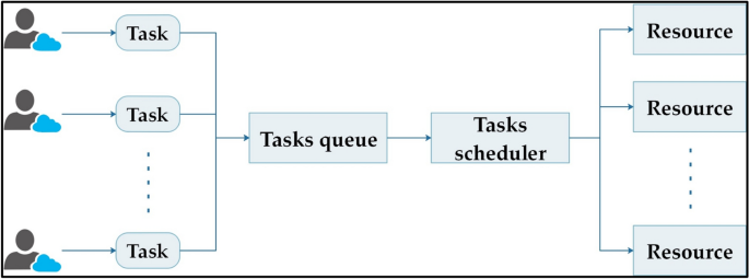
Task resource allocation diagram.
The issue with job scheduling can be summed up like this: You need to allocate minutes to a task while keeping an eye on your resource budget, making sure everything gets done within the set timeframe. Also, figure out the costs and the time required to finish the job. Remember, the project’s budget limit is budgeting B. Find the minimum cost to complete the project. If the minimum construction time after project completion exceeds deadline D or the minimum construction cost exceeds budget B, the project plan will not be met. To distribute tasks to appropriate resources to reduce delivery time and cost, therefore, the problem is defined as follows.
Definition 1
The \(n\) tasks submitted by the user are described by a Directed Acyclic Graph \(\left(DAG\right)G = \left(T, E\right),\) where \(T = \left\{t1, t2, \dots , tn\right\}\) represents a task set with \(n\) tasks and \(E = \left\{{e}_{ij}\right\}\) is an edge set, which represents the dependency relationship between tasks. If \({e}_{ij}= 0\), The analysis indicates that there’s no connection between the execution sequences of tasks ti and tj. When eij equals 0, it suggests that task tj can be finished only after task ti is done. Additionally, the value of eij shows how much data needs to be transferred between these two tasks, ti and tj.
Definition 2
The available resources in the cloud computing system are represented by \(R = \{r1, r2, …, rm\},\) where \(m\) is the number of resources.
Definition 3
The matrix \(W = T * R\) is all about the time costs involved in processing tasks, where \({w}_{ij}\) indicates how long it takes to handle task \({t}_{i}\) on resource \({r}_{j}\).
Definition 4
The matrix \(C = R * R\) looks at the communication or data transfer capacity between two resources. Here, the variable \({c}_{ij}\) shows how well resource \({r}_{i}\) can transmit data to resource \({r}_{j}.\)
Definition 5
We refer to the method for allocating tasks to resources as X. The way we allocate a specific set of tasks T to a set of resources R is outlined in Eq. 1 below.
$$X(n,m) = \{x11,x12,…,x1m,x21,x22,…,xik,…,xnm\}$$
(1)
where \({x}_{ij} = \text{0,1}\), indicating whether to assign task \({t}_{i}\) to resource \({r}_{j}\). Then, the Total Processing Time (TPT) of all tasks is calculated as follows:
$$TPT=\sum_{i=1}^{n}\sum_{j=1}^{m}{x}_{ij}{w}_{ij}$$
(2)
TPT represents the total processing time spent when all tasks are assigned to appropriate processing resources, and \({x}_{ij}{w}_{ij}\) represents the processing time of task \({t}_{i}\) assigned to resource \({r}_{j}\). According to Eq. 2, the total processing cost of all tasks is calculated as follows as Eq. 3:
$$cost=\sum_{i=1}^{n}\sum_{j=1}^{m}{x}_{ij}{w}_{ij}{price}_{j}$$
(3)
where cost indicates that the total processing cost of the task is equal to the product of the processing time of each task and the unit time price \({price}_{j}\) allocated to a specific resource. The \({price}_{j}\) represents the cost spent by resource \({r}_{j}\) to perform the task in unit execution.
According to the task allocation strategy \(X\), it can be concluded that task \({t}_{i}\) is assigned to resource \({r}_{k}\) for processing; task \({t}_{i}\) is assigned for resource \({r}_{l}\) to execute; then for all tasks, the total data transmission time \(DTT\) is calculated as follows:
$$DTT= \sum_{i=1}^{n}\sum_{j=1}^{m}\frac{{e}_{ij}}{{c}_{kl}}$$
(4)
According to Eqs. 2 and 4, it can be concluded that the maximum completion time make span of all tasks is calculated as follows:
$$makespan = S + TPT + DTT$$
(5)
The total time it takes to complete all tasks is made up of three parts: the time spent searching for resources (S), the processing time for each task (TPT), and the overall data transmission time (DTT). Based on the study mentioned earlier, the task resource allocation model can be mathematically defined as finding the best way to allocate a given set of resources (R) to a set of tasks (T) so that once the tasks are assigned to the resources, the task completion time and execution cost minimum. According to Eqs. 3 and 5, the objective function is defined as follows:
$$func = cost + makespan$$
(6)
The purpose of Eq. 6 is to minimize the cost, and its constraints are:
Constraints state that budget and time constraints can be maintained while minimizing costs and time to completion. According to Eqs. 3, 5, and 6, to achieve the optimization goal, the main factors that affect the optimization goal are the resource search time \(S\) in Eq. 5, the execution completion time of all tasks \(TEFT\) and the time of all tasks. The total data transmission time \(DTT\) is mainly affected by the scheduling algorithm itself. Therefore, how to reduce the values of \(S,\) \(TEFT\), and \(DTT\) is the primary consideration of the scheduling algorithm.
Task scheduling strategy based on HEFT algorithm
The HEFT algorithm35 which focuses on selecting the most important tasks and assigning the necessary processing resources to them when used in a heterogeneous distributed environment, is a clever way to schedule a wide range of resources. Its main objective is to decrease the amount of time required to complete activities, and it has been successful in lowering the earliest task scheduling completion time.
HEFT algorithm process
The HEFT algorithm process consists of three key phases: selecting resources, assigning task priorities, and determining weight assignments. During the task priority assignment phase, we establish the priority for each path, create a list based on that priority, and then derive a task list from the prioritized paths before scheduling the tasks. Meanwhile, the weight assignment phase primarily focuses on updating the relevant node or edge weights. This method ensures that resources are allocated to tasks based on the principle of assigning each job to the resource node that can complete it the quickest.
Weight assignment stage
Since the resources allocated to tasks have different values in terms of CPU, memory, disk space, etc., the original weight of edges between tasks cannot accurately reflect their priority. It needs to be based on the computing and transmission performance of resources. Task nodes and edges between tasks are given new weights.
Definition 6:
Use an undirected graph \(RG = \left(R, C\right)\) to describe resources, where R represents a collection of resources, which has been specifically described in definition 2, where \({r}_{i}\) represents the computing performance of the \(ith\) resource;
\(C = \{c11,c12,…,c1m,c21,c22,…,cmm\}\) represent the edges between resources and the data transmission capability between resources.
The average computing performance of the resource collection is as follows:
$$compute= \frac{\sum_{i=1}^{m}{r}_{i}}{m}$$
(9)
According to Eq. 9, the computing performance heterogeneity factor is calculated as follows:
$$compute= \frac{\sqrt{\sum_{i=1}^{m}({r}_{i}-compute)}}{m\times {i\le m}^{\text{max}{r}_{i}}}$$
(10)
Use \(\eta\) to measure the difference in resource computing performance. The smaller the value of \(\eta\), the smaller the difference between resources and the average transmission performance between resources is as follows:
$${\text{trans}} = \frac{{\sum\nolimits_{i = 1}^{m} {\sum\nolimits_{j = i + 1}^{m} {c_{ij} } } }}{m(m – 1)/2}$$
(11)
According to Eq. 11, the transmission performance heterogeneity factor is calculated as follows:
$$trans = \frac{{\sqrt {\sum\nolimits_{i = 1}^{m} {\sum\nolimits_{j = i + 1}^{m} {(c_{ij} – trans)} } } }}{{m(m – 1)/2 \times \max_{i,j \le m} c_{ij} }}$$
(12)
Use \(\delta\) to measure the difference in transmission performance between resources. The larger the value of \(\delta\), the greater the difference in transmission performance between resources.
According to Eqs. 10 and 12, the new weight \({t}_{i}{\prime}\) of task nodes and the new weight \({e}_{ij}{\prime}\) of edges between tasks can be calculated as follows:
$$t^{\prime}_{i} = \frac{{t_{i} }}{{\eta \min_{j \le m} r_{j} + (1 – \eta )\max_{j \le m} r_{j} }}$$
(13)
$$e^{\prime}_{ij} = \frac{{e_{ij} }}{{\delta \min_{x,y \le m} c_{xy} + (1 – \delta )\max_{x,y \le m} c_{xy} }}$$
(14)
According to Eqs. 13 and 14, update the task node and edge weights between task nodes.
Priority assignment phase
To figure out the priority of each path in the task-directed graph, you’ll need to use the updated weights for the task nodes and the edge weights that link them. The paths are then organized by their priority values, from highest to lowest, creating a list that can be handy for scheduling tasks down the line.
The priority \(rank\left(pk\right)\) for path \({p}_{k}\) is calculated as follows:
$$rank(pk) ti\in pk = X (t{\prime}i + e{\prime}i,succ(i))$$
(15)
The priority \(rank\left(pk\right)\) of path \({p}_{k}\) equals the weight of all tasks \({t}_{i}\) on the path and the sum of the weights of the edges between task \({t}_{i}\) and its successor tasks. After the path list is formed, the subsequent task scheduling operation will start from the path with higher priority in the path list. When scheduling task \({t}_{i}\) in the path, all the predecessor tasks of task \({t}_{i}\) have been scheduled; then, task \({t}_{i}\) will be inserted into the task scheduling list until all tasks are selected.
Resource allocation phase
When task \({t}_{i}\) needs to be scheduled for execution, it is necessary to calculate the earliest completion time \(EFT ({t}_{i},{r}_{j})\) of task \({t}_{i}\) on each resource \({r}_{j}\). For this purpose, calculate the earliest start time \(EFT ({t}_{i},{r}_{j})\) of task \({t}_{i}\) placed on resource rj and free time slot \(({t}_{i},{r}_{j})\).
For the earliest start time \(EFT ({t}_{i},{r}_{j})\) of task \({t}_{i}\) assigned to resource \({r}_{j}\), the calculation formula is as follows:
$$EST(t_{i} ,r_{j} ) = \max \{ avail(r_{j} ),\max_{{t_{k} \in pred(t_{i} )}} \{ EFT(t_{k} ,r_{q} ) + dtt(k,i)\} \}$$
(16)
To determine the earliest start time (EST) for task \({t}_{i}\), we first need to find the maximum value of the sum of the data transmission time, which is represented as max \(\left\{EFT \left(tk,rq\right)+dtt\left(k, i\right)\right\},\), along with the earliest completion time of its predecessor task. Once we have that maximum value, we can use it as the EST for task \({t}_{i}\), but only after comparing it with the initial load time avail(\({r}_{j}\)) of resource \({r}_{j}\) for all predecessor tasks \(\text{tk}\in \text{pred}\left(\text{ti}\right)\). It’s important to note that the earliest start time for the entry node is \(EST (tentry, {r}_{j}) = 0\). Meanwhile, \(avail({r}_{j})\) refers to the initial load time of the resource, which indicates when the resource is ready to take on the next task after completing its current assignments. The set of parent tasks for task \({t}_{i}\) is denoted as pred(\({t}_{i}\)). Lastly, the data transmission time between task tk and task \({t}_{i}\), or \(dtt(k, i)\), is calculated directly, assuming that job tk is assigned to resource \({r}_{x}\).
$$dtt(k,i) = \frac{{e_{ki} }}{{c_{xj} }}$$
(17)
The earliest completion time EFT(ti,rj) of task ti on resource rj is calculated as follows:
$$EFT(ti,rj) = EST(ti,rj) + wij$$
(18)
Then, the earliest completion time EFT is equal to the sum of the earliest start time EST of the task and the execution time of the task resource. The free time slot \(slot(ti,rj)\) describes the waiting time of task \(ti\) on resource \(rj\), and its calculation is as follows:
$$slot(ti,rj) = EST(ti,rj) – avail(rj)$$
(19)
When calculating the earliest start time \(EST(ti,rj)\) of task \(ti\) placed on resource \(rj\) and the free time slot \(slot(ti,rj)\), it is necessary to determine whether task \(ti\) has an unexecuted predecessor task and, if so, whether the predecessor task tk satisfies:
Condition 1:
$$slot(ti,rj) \ge w(k,j)$$
(20)
Condition 2: Resource \(rj\) never executes task \(tk\). When task \(ti\) meets the above conditions, insert it into the free time slot and update its \(EST (ti,rj)\) and \(slot(ti,rj)\) on the resource. Execute the above condition judgment in a loop until the condition is not satisfied or the predecessor task has been executed. At this time, calculate the earliest completion time \(EFT (ti,rj)\) of task \(ti\) on resource \(rj\) according to Eq. 18.
The earliest completion time \(EFT (ti,rj)\) of task \(ti\) on each resource \(rj\) is calculated by the above method, and compared the resource with the shortest earliest completion time is selected for task execution. When the task queue is empty, the resource allocation process ends.
HEFT-based task scheduling algorithm
The HEFT method uses a combination of resource allocation, weight allocation, and priority calculation to figure out which job should take precedence for effective task scheduling. Here’s a quick rundown of the steps involved in executing the algorithm:
Algorithm 1: HEFT algorithm
-
i.
Input the workflow and convert it into a directed acyclic graph DAG;
-
ii.
Update task node weights and weights of edges between tasks according to Eq. 13 and Eq. 14;
-
iii.
Calculate the priority of the DAG graph path according to Eq. 15;
-
iv.
Construct a path list according to the path priority;
-
v.
Build a task list based on the path list;
-
vi.
Make sure to finish every task on your list;
-
vii.
Go through each resource in the collection to check if the previous task has been completed;
-
viii.
If the task before it isn’t done yet, it will keep checking to see if it meets Conditions 1 and 2 and whether it’s finished; if it’s not, it will break out of the loop; if it is, it will jump straight to the next step;
-
ix.
Look for the earliest expected finish time (EFT) for the task on this resource;
-
x.
Choose the resource that can complete the task the quickest, assign the tasks, and update the task list once you’ve gone through all the resources.
Algorithmic analysis
During the scheduling process, HEFT assigns tasks to resources by looking at the earliest completion time for each available resource. It hands out assignments to the resource that can finish the earliest, which helps to reduce the overall completion time. However, while HEFT is quite effective, it does come with some drawbacks. One major issue is that figuring out the earliest completion time for every task across all resources adds to the computational complexity of the HEFT method. This exhaustive computation process results in a vast resource search space and incurs high resource search costs. Consequently, the algorithm may need help with scalability, mainly when scheduling workflows of considerable size or complexity. Its pursuit of minimizing completion time, the HEFT algorithm overlooks the user’s requirements regarding task execution costs. While prioritizing completion time optimization is crucial, the algorithm’s failure to account for users’ varying cost constraints or preferences may lead to suboptimal resource allocations. This limitation becomes particularly pronounced when users prioritize cost-effectiveness or have specific budget constraints that must be addressed during task execution.
Hierarchical task scheduling strategy
The HEFT method tackles the task serial scheduling problem by using list scheduling to ensure tasks are completed as quickly as possible. However, this approach comes with its downsides. The serial scheduling strategy of the HEFT algorithm can lead to high computational costs, as it searches for all resources in a broad manner, which drives up the resource search expenses. Additionally, it doesn’t take the budget cost factor into account during task scheduling, making it less practical. To address the issue of resource search costs, this section introduces a resource preprocessing technique to enhance the HEFT algorithm through hierarchical task scheduling. It introduces a segmented scheduling mechanism to enable HEFT to achieve parallel scheduling of tasks and save task execution time. Budget and time constraints are introduced in the HEFT algorithm to minimize the task execution cost.
Resource preprocessingCloud resource fuzzy clustering
This section uses fuzzy clustering to preprocess cloud computing resources. The decentralized and independent cloud computing resources are divided into several categories according to their characteristics to solve the problems of low efficiency, resource waste, and high time complexity caused by the large search space of task scheduling resources. Clustering is dividing objects according to their characteristic similarity and dividing objects with similar characteristics into the same class. Currently, research on clustering methods mainly focuses on merging, partitioning, and modeling. Clustering methods are also widely used. When the clustered objects have distinct group characteristics, the clustering process will strictly divide specific objects into a particular class according to the objective function, and the relationship between objects and classes only exists between inclusion and non-inclusion. However, most objects that need to be clustered show outstanding individual characteristics, and their class relationship is not clear when they are divided, so fuzzy clustering is required. In the cloud computing environment, cloud resources have characteristics such as uncertainty and diversity. It is necessary to use the fuzzy clustering method to divide cloud computing resources into different categories according to the multiple characteristics of resources to assign different tasks to different types of resources. In the cloud computing environment, the fuzzy clustering model is shown in Fig. 2.
Fig. 2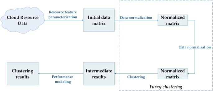
Fuzzy clustering is mainly the process of processing resource feature matrices. The completed fuzzy clustering process first needs to collect the data of cloud computing resources and establish the initial data matrix according to the characteristic attributes of the resources. The initial matrix describes the multi-attribute characteristics of each resource. Due to the differences in the order of magnitude and dimension of the characteristic attributes of each resource, it is necessary to transform the initial data matrix properly, that is, to standardize the data, standardize the value of each characteristic attribute to a specific range, and eliminate the influence of the order of magnitude on subsequent calculations. The data normalization operation limits the range of values in the standard matrix between 0 and 1, which is convenient for subsequent clustering.
Resource fuzzy clustering process
This paper uses \(S = \{s1, s2, …, sM\}\) to represent the collection of resources to be clustered, where \(M\) represents the number of resources; use the vector \(S{\prime}(si) = \{si1,si2,…,siv\}(i = \text{1,2},…, M)\) represent the characteristic attribute of the \(ith\) resource, where \(sij\) represents the \(jth\) characteristic attribute of the \(ith\) resource. \(V\) represents the number of characteristic attributes. Each computing resource \(sn\) in the set \(S = \{s1, s2, …, sM\}\) has a model vector \(S{\prime}(si) = \{si1,si2,…,siv\}(i = \text{1,2},…, M)\) represents the characteristic attribute of the \(ith\) resource, where \(sij\) represents the value of the \(ith\) computing resource on the \(jth\) quality attribute. The characteristics of cloud computing resources mainly include computing power, data transmission capacity, memory size, storage capacity, data transmission capacity limit, network location, number of connections, etc., and clustering cloud computing resources according to their characteristic attributes will have similar characteristics. The choice of attribute characteristics is crucial when grouping resources. In this section, \(v = 4\) is selected, indicating that cloud computing resources have four characteristics, which are defined as follows:
The computing performance of resource nodes refers to the average processing power available within a cloud computing system, and we denote this performance with the term t1. This computing performance is closely tied to how long it takes to execute jobs, significantly influencing the time costs involved in task scheduling.
On the other hand, t2 represents the system’s data transmission capability. We can think of the average edge weights between resources, or the average communication capabilities of the connections, as a way to describe how well data is transmitted between resources in a cloud computing environment. The level of performance in data transmission directly impacts the time it takes to transfer data between different processes.
\(t3\) represents its maximum transmission capacity. In the cloud computing system, the maximum amount of data is transferred between resources each time. The number of data transfers per time directly affects this.
\(t4\) represents its link number. In cloud computing, multiple resources are connected to this resource node. Tasks assigned to this resource can perform data transfers with tasks from multiple other resources.
The rest of the feature tasks have little impact on the scheduling performance and are not considered here. If too many feature attributes are considered, the fuzzy clustering process’s time complexity will be too high, which deviates from the purpose of this paper.
This paper’s fuzzy clustering resource preprocessing procedure has four steps: normalization of the experimental data range, realization of the fuzzy matrix, and evaluation of clustering information.
1) Normalize the range of experimental data:
The primary purpose of this step is to eliminate the effect of magnitude on subsequent calculations. To obtain standardized data for the original data S′, the normalized value \(p_{ik}^{\prime }\) of each data is calculated as follows:
$$p_{ik}^{\prime } = \frac{{p_{ik} – \overline{{t_{k} }} }}{{\sigma_{{t_{k} }} }}$$
(21)
where \(tk\) represents the \(kth\) eigenvector in \(S\)′ \(tk\) is the mean of \(tk\). \(\sigma tk\) is the standard deviation of tk. Since the standardized value \(p_{ik}^{\prime }\) is not all in \([\text{0,1}],\) we use the range standardization method to transform \(S{\prime}\) into \(S{\prime}{\prime}\). The range normalization method is defined as follows:
$$p_{ik}^{\prime \prime } = \frac{{p_{ik}^{\prime } – p_{k\min }^{\prime } }}{{p_{k\max }^{\prime } – p_{k\min }^{\prime } }}$$
(22)
where \({p}{\prime}kmin\) and \({p}{\prime}kmax\) are the minimum and the maximum values \(p_{1k}^{\prime } ,p_{2k} , \ldots p_{Nk}^{\prime }\), respectively.
2) Fuzzy matrix implementation:
The main goal of this stage is to help organize resources in the future based on how similar their cloud computing features are. Using the exponential similarity coefficient approach, the fuzzy similarity relation \(Rs\) of the processing unit \(S = \{s1, s2, …, sN\}\) may be determined as follows:
$$r_{ij} = \frac{1}{N}\sum\limits_{k = 1}^{N} {e^{{ – \frac{{3(p_{ik} – p_{jk} )^{2} }}{{S_{tk}^{\prime \prime 2} }}}} }$$
(23)
Among them \(S_{tk}^{\prime \prime 2}\) is the variance of the kth feature, and rij is the similarity between processing units pi and pj. At the same time, the fuzzy equivalence relation Re with transitive closure is obtained through the synthesis operation of the similarity coefficient matrix.
(3) Evaluate the clustering information with the evaluation function:
Use the merit function to estimate the clustering results. Set different values for the cutset level alpha to get different clustering results. A higher degree of resemblance between clusters is indicated by an alpha value near 1, whereas a lesser degree of similarity is indicated by an alpha value close to 0. In this paper, according to the historical experimental data, α = 0.8 can get a better clustering result, and at this time, the cut set \(Rg\) is obtained.
The clustering result can be obtained through the \(Rg\) matrix, represented by \(CLUSTER = \{CL1, CL2, …, CLK\}\). In this case, the overall performance of each cluster can be estimated as follows:
$$PERF(CL_{j} ) = \frac{1}{w}\sum\limits_{{p_{w} \in CL_{j} }} {\sum\limits_{i = 1}^{n} {\alpha_{i} } } P^{N} [k][i$$
(24)
where w is the cluster’s total number of processing units, \(CLj\) represents the \(jth\) cluster, and the value of \(alphai\), which denotes the weight of the processing unit’s \(ith\) feature, can often be determined using historical data or experimental results. By calculating the overall performance of each cluster, the updated \(CLUSTER = \{CL1, CL2, …, CLK\}\) can be obtained, where \(CL1, CL2,…, CLK\) are sorted according to their performance. The clustering flowchart is shown in Fig. 3.
Fig. 3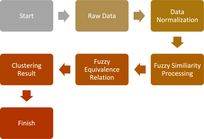
Fuzzy clustering flow chart.