Transduction parameter
We consider the dynamics of a string of N trapped ions perturbed by an external electric field, which results in a force δFj(t) = −qδEj(t) on ion j. Restricting ourselves to a single direction without loss of generality, the Lagrangian of this system is53
$$\begin{aligned}{{L}}&=\frac{{{m}}}{2}\left(\sum_{{{p}}=1}^{{{N}}}{(\dot{Q}_{p}({{t}}))}^{2} – {\nu}_{{{p}}}^{2}{{{{Q}}}_{{{p}}}}^{2}({{t}})\right)\\ &\quad{}+{{q}}{{{Q}}}_{{{p}}}({{t}})\sum_{{{j}}=1}^{{{N}}}{{{b}}}_{{{j}}}^{({{p}})}\delta {{{E}}}_{{{{j}}}}({{t}}),\end{aligned}$$
(7)
where νp are the normal mode frequencies and \({{{b}}}_{{{j}}}^{({{p}})}\) describes how strongly ion j couples to the mode p. The normal modes of motion Qp(t) are related to small displacements of the ion, δr(t) of equation (1), via:
$${{{Q}}}_{{{p}}}({{t}})=\sum_{{{j}}=1}^{{{N}}}{{{{b}}}_{{{j}}}}^{({{p}})}\delta {{r}}({{t}}).$$
(8)
The equation of motion of the pth normal mode is found from the Lagrangian using the relation
$$\frac{\rm{d}}{\rm{d}t}\left(\frac{\partial {{L}}}{\partial \dot{Q}_{p}(t)}\right)=\frac{\partial {{L}}}{\partial Q_{p}(t)},$$
resulting in
$${\ddot{{{Q}}}}_{{{p}}}({{t}})+{\nu}_{{{p}}}^{2}{{{Q}}}_{{{p}}}({{t}})=\frac{{{e}}}{{{m}}}\sum_{{{j}}=1}^{{{N}}}{{{b}}}_{{{j}}}^{({{p}})}\delta {{{E}}}_{{{j}}}({{t}}).$$
(9)
Without loss of generality, we restrict ourselves to a single-ion chain, N = 1, and consider the centre-of-mass motion along the z axis. After setting p = z and \({{{b}}}_{1}^{(1)}=1\), equation (9) becomes
$${\ddot{{{Q}}}}_{{\rm{z}}}({{t}})+{\nu}_{{\rm{z}}}^{2}{{{Q}}}_{{\rm{z}}}({{t}})=\frac{{{e}}}{{{m}}}\delta {{E}}({{t}}).$$
(10)
This corresponds to the equation of a driven harmonic oscillator. Taking the Fourier transform, equation (10) becomes
$${\hat{{{Q}}}}_{{{p}}}(\omega)=\frac{{{e}}}{{{m}}({\nu}_{{\rm{z}}}^{2}-{\omega}^{2})}\delta \hat{{{E}}}(\omega),$$
(11)
where \(\hat{\cdot }\) denotes the Fourier transform. For N = 1 ion, Qp(t) = δr(t) and equation (11) becomes
$$\delta \hat{{{r}}}(\omega)=\frac{{{e}}}{{{m}}({\nu}_{{\rm{z}}}^{2}-{\omega}^{2})}\delta \hat{{{E}}}(\omega).$$
(12)
In the limit νz ≫ ω, equation (12) reduces to
$$\delta \hat{{{r}}}(\omega)=\frac{{{e}}}{{{m}}{\nu}_{{\rm{z}}}^{2}}\delta \hat{{{E}}}(\omega),$$
(13)
from which one can retrieve the expression of equation (1). From equation (12), we also find that the coupling of radial micromotion into the spin states is negligible. These oscillations occur at the RF trap frequency, ΩRF/2π = 19.22 MHz, and the resulting amplitude of the radial oscillation is negligible because ΩRF ≫ νx,y.
Experimental set-up
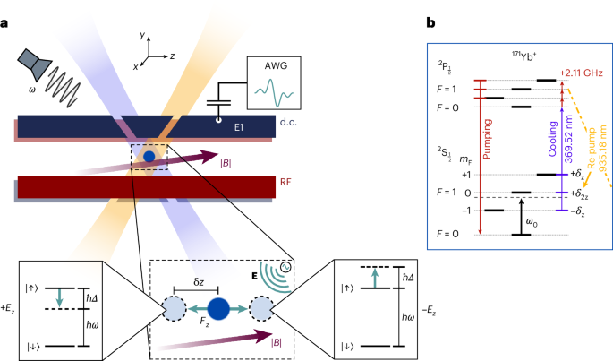
Extended Data Fig. 5 shows a schematic of the experimental set-up used in this work. The ion trap was mounted inside a vacuum chamber maintained at an average pressure of 2.4 × 10⁻¹¹ mbar. The ion is Doppler cooled using a 369.52 nm laser that is red-detuned from the 2S1/2 |F = 1〉 to the 2P1/2 |F = 0〉 transition. The laser beam is double-passed through an acousto-optic modulator to allow for fine frequency and amplitude control by a field-programmable gate array. An electro-acoustic modulator (EOM) is used to generate 2.11 GHz sidebands for state preparation. These sidebands allow the population to be driven into the 2P1/2 |F = 1〉 state via optical pumping, after which it decays into the |↓〉 = 2S1/2 |F = 0〉 ground state. The population that is off-resonantly driven into the 2S1/2 |F = 0〉 state during Doppler cooling is returned to the cooling cycle by continuously applied microwaves near 12.64 GHz. Population can also leak out of the Doppler cooling cycle by decaying into the 2D3/2 manifold, where a 935.18 nm re-pump laser applied on the 2D3/2 to 3D[3/2]1/2 transition returns population to the 2S1/2 |F = 1〉 state. The re-pump laser is also modulated by an EOM at 3.07 GHz to improve the re-pumping efficiency. Microwaves are generated by a vector signal generator (Keysight E8267D PSG), which produces a carrier signal of 12.54 GHz. This is then mixed with RF pulses near 100 MHz generated by a two-channel AWG (Keysight M8190A), which is then amplified and emitted by an external microwave emitter to allow for coherent manipulation of the spin state. The spin state is measured using a state-dependent fluorescence scheme as described in ref. 50. The average SPAM error was found to be η = 1.8 × 10⁻². The voltage signals used to measure the a.c. and d.c. sensitivities are applied directly to the capacitor from the second channel of the AWG. To measure the electric field noise, a white-noise waveform is generated using a separate AWG (Agilent 33522A). The white-noise signal is attenuated by two 30 dB RF attenuators, and its output controlled with an external RF switch.
Gradient measurement
The strength of the magnetic field gradient along the axial direction was calculated by measuring the transition frequencies of two co-trapped 171Yb+ ions. As the splitting of the 171Yb+ spin states is dependent on the strength of the magnetic field at the position of the ion, the magnetic field gradient in the axial direction is given by
$$\frac{\partial {{B}}}{\partial {{z}}}=\frac{{{{B}}}_{2}-{{{B}}}_{1}}{\delta {{Z}}},$$
(14)
where B1 and B2 are the magnetic field strengths at the location of each ion, and δZ is the ion separation (Extended Data Fig. 1). The ion separation is a result of the mutual Coulomb repulsion between the ions and the oppositely acting axial confinement force. δZ is given by53
$$\delta {{Z}}={\left(\frac{{e}^{2}}{4\uppi {\epsilon}_{0}{{m}}{\nu}_{\rm{z}}^{2}}\right)}^{1/3}\frac{2.018}{{{{N}}}^{0.559}},$$
(15)
where νz is the axial vibrational centre-of-mass frequency, m is the mass of a single charged particle and N is the number of ions in the crystal. We measured νz/2π = 161.191(8) kHz via the ‘tickling’ method. An a.c. electric field was applied to the trap using an external RF coil, which excites the axial motion of the ion crystal when the applied frequency is resonant with the axial vibrational frequency, leading to a measurable decrease in ion fluorescence due to the Doppler shift. We then compute δZ = 12.64(1) μm from equation (15).
The magnetic field at each ion was calculated by measuring the magnetic field-dependent transition frequency of each ion, as shown in the inset plots of Extended Data Fig. 1. From these measurements, B1 = 7.1328(8) G and B2 = 9.9655(5) G. Finally, from equation (14), the magnetic field gradient strength was ∂B/∂z = 22.41(1) T m−1.
Calibrating α and γ
The geometric factor of an electrode, α, relates the electric field at the position of the ion to the voltage applied to the electrode, and is defined as
$$\alpha =\frac{\partial {{E}}}{\partial {{V}}}=\frac{\partial \omega}{\partial {{V}}}\frac{\partial {{E}}}{\partial {{z}}}{\left(\frac{\partial {{B}}}{\partial {{z}}}\frac{\partial \omega}{\partial {{B}}}\right)}^{-1},$$
(16)
where ∂E/∂z = mνz2/e. We calibrate α by first measuring the change in magnetic field at the ion due to a change in the voltage applied to the E1 electrode (∂B/∂V) using the second-order sensitive spin state transition frequency and νz/2π = 161.191(8) kHz (Extended Data Fig. 2). The measurement was performed with a single 171Yb+ ion by applying a voltage V0+δV to the electrode, where V0 = 1.75 V is the static voltage contributing to the axial confining potential and δV is an offset that is varied from −50 to +50 mV. We extract the value of ∂B/∂V from a least squares fit to a straight line of the magnetic field measurements for each voltage offset. From this, we then determine
$$\frac{\partial \omega}{\partial {{V}}}=\frac{\partial {{B}}}{\partial {{V}}}\frac{\partial \omega}{\partial {{B}}}=-382\times 1{0}^{3}\,{\rm{rad}}\,{{\rm{V}}}^{-1}.$$
The geometric factor is then calculated from equation (16), giving α = −95.64(4) m−1.
The transduction parameter is found using
$$\gamma =\frac{1}{\alpha }\frac{\partial \omega }{\partial {{V}}}=\left(\frac{\partial {{V}}}{\partial {{E}}}\frac{\partial \omega }{\partial {{V}}}\right).$$
For the second-order magnetic field sensitive transition, we measure γ = 3,998(2) rad m V−1.
Our scheme measures the electric field component along the z axis, as the sensitivities to electric fields in the x and y axes are negligible. To see this, we calculate the ratio between the transduction parameter in the z direction, γ = γz, and the transduction parameter in the x and y directions, γx,y, using equation (2). The magnetic field gradient along the z axis was measured to be ∂B/∂z = 22.41(1) T m−1, whereas the gradient along the x and y axes was estimated through numerical simulations to be ∂B/∂rx,y ≈ 11 T m−1. With the motional frequencies νz/2π = 161.191(8) kHz and νx,y/2π ≈ 1.5 MHz, the ratio of the transduction parameters is
$${\gamma}_{{\rm{z}}}/{\gamma}_{{\rm{x}},{\rm{y}}}=\frac{\partial {{B}}}{\partial {{z}}}\frac{\partial {{z}}}{\partial {{{E}}}_{{\rm{z}}}}\left/\frac{\partial {{B}}}{\partial {{{r}}}_{{{\rm{x}}},{\rm{y}}}}\frac{\partial {{{r}}}_{{{\rm{x}}},{\rm{y}}}}{\partial {{{E}}}_{{{\rm{x}}},{\rm{y}}}}\approx 180,\right.$$
which indicates that the sensitivity to electric fields in the radial direction is over two orders of magnitude weaker.
Electric field sensing protocol
For the sensing of a.c. fields, we follow the pulse sequence protocol outlined in ref. 35 and illustrated in Extended Data Fig. 3. The a.c. sensing sequence is realized by first initializing the two-level system into the \(\vert +\rangle =({1}/{\sqrt{2}})(\vert \downarrow \rangle +\vert \uparrow \rangle )\) state using a π/2 pulse. The superposition state then evolves under an electric field perturbation for a time τ/2. A π pulse reorients the spin along the equator of the Bloch sphere, before the quantum state again evolves under the electric field perturbation for a time τ/2. A final π/2 pulse mapps the state population into the σz basis for detection. Using this pulse sequence, the sensitivity of the spin state transition frequency is maximized for a.c. signals oscillating at a frequency of τ−1.
The d.c. sensing experiments also use a Hahn echo type pulse sequence, whose benefits are twofold. First, the coherence time of the sensor is greatly extended when compared to that of the Ramsey-type sequence, which allows for increased sensitivities. Second, the refocusing π pulse also compensates for detuning errors in the microwave pulses. The pulse sequence is illustrated in Extended Data Fig. 3, and begins with a π/2 pulse to initialize the spin into the \(\vert +\rangle =({1}/{\sqrt{2}})(\vert \downarrow \rangle +\vert \uparrow \rangle )\) state. d.c. signals cannot be applied through a capacitor. The low-pass filter signal chain of the d.c. electrode is also not suitable for fast application of d.c. square pulses during the sensing pulse sequence, as the low-pass filter would significantly attenuate and distort the signal. Therefore, to quantify the sensor’s response to d.c. signals, we apply an a.c. signal of frequency τ−1 for the duration of the first τ/2 delay time. This corresponded to an equivalent d.c. voltage on the electrode of Vd.c. = (2/π)VPK, where VPK is the amplitude of the applied signal. Here, (2/π)VPK is the average voltage over the half-oscillation of the a.c. waveform. The applied time-varying pulse therefore causes the spin state to accumulate the same amount of phase ϕ as a square d.c. pulse of amplitude (2/π)VPK applied for a duration τ/2 based on the equation relating phase accumulation to the detuning of the spin transition: \(\phi =\int_{0}^{{\tau}/{2}}\gamma \alpha \delta {{V}}({{t}})\,\mathrm{d}t\). The refocusing π pulse is then applied, followed by the second τ/2 delay time, during which no other voltage signals are applied to the electrode, followed by a final π/2 pulse.
In addition to the electric field interaction time τ, the second relevant time parameter from equation (4) is tm, which breaks down as follows for our experimental implementation: (1) d.c. offset application delay time, 50 ms (see next section), (2) Doppler cooling and detection, 14.599 ms, (3) state preparation and microwave pulses, 2.155 ms and (4) data processing and field-programmable gate array delays, 85 μs. The total tm = 66.839 ms.
Capacitive coupling of a.c. signals
Due to the absence of an in-vacuum antenna, the electric field signals measured by the trapped ion were emitted from an in-vacuum end-cap electrode, which also generated a d.c. confinement electric field. Voltage waveforms were generated by an AWG and capacitively coupled onto the electrode across a 220 pF capacitor. Due to their frequency-dependent impedance, capacitors act as high-pass filters, thereby attenuating the lower-frequency signals more strongly. The fixed response time of a capacitor will also shift the phase of a.c. signals that are applied across it. This shift in phase of the a.c. signal can, if unaccounted for, affect the total coherent phase ϕ that is accumulated by the spin states. To achieve an optimal measurement of the sensitivity of our experimental system, it is necessary for the electric field signal at the ion to be in phase with the Hahn-echo sensing pulse sequence. This is because ϕ is the difference between the coherent phase accrued during the first and second interaction times τ/2. An electric field signal that is not in phase with the Hahn-echo sequence will, therefore, reduce the measured sensitivity. References 11 and 35 provide further information about this effect.
We measure the phase shift on signals applied across the capacitor for the span of frequencies used in the a.c. and d.c. sensing experiments using an oscilloscope. Based on these measurements, we then pre-compensate the signal applied across the capacitor by applying an inverse phase shift, negating the effect of the capacitor on the phase of the voltage waveform. This ensures that the voltage on the electrode and, therefore, the electric field signal at the ion, are in phase with the Hahn-echo sequence.
Shifting the phase of the voltage waveform introduces a discontinuity into the signal. This manifests as a sudden change in the voltage across the capacitor from 0 to VΦ = VA sin Φ, where Φ is the phase of the a.c. voltage signal. Given that the current across a capacitor is defined as I = C dV/dt, where C is the capacitance of the capacitor, the high rate of change of voltage induces a large current flow across the capacitor, which introduces additional coherent phase offsets of the superposition state. To suppress this unwanted perturbation, we apply a d.c. voltage offset of VΦ into the capacitor in the time before the initialization of the |+〉 state, which minimized the sudden voltage spike across the capacitor from the phase-shifted a.c. voltage waveform. To ensure that the sensor reaches a steady state before the application of the a.c. electric field signal, an extra 50 ms delay is added between the application time of the d.c. offset and the first resonant microwave pulse. This made up most of the tm time, which was broken down in the previous section. The pre-compensation technique for the a.c. and d.c. sensing pulse sequences is visualized in Extended Data Fig. 3, which illustrates both the AWG and in-vacuum electrode voltage evolution throughout the experimental pulse sequence.
We also measure the frequency-dependent attenuation of the capacitor using an oscilloscope. We determine the transfer function of the capacitor by fitting a Butterworth high-pass filter function to these data. We then find the total attenuation of the electric field signal for a given frequency τ−1.
Determination of the coherence time
We measure the coherence time of the two-level system using a Hahn-echo experiment. The spin is initialized in the |↓〉 state, after which a π/2 pulse rotates the spin into the |+X〉 eigenstate. A refocusing π pulse is applied between the two free evolution periods of duration τ/2. A final π/2 pulse maps the state into the σz basis for detection. Varying the phase of the final pulse from −2π to 2π results in sinusoidal fringes in the probability of measuring |↑〉. As the free evolution time is increased, decoherence leads to a reduction in the amplitude of these fringes. The coherence time T2 is given by the point at which the fringe contrast reaches e−1. As the a.c. and d.c. sensing experiments were also based on the Hahn-echo sequence, the fringe amplitudes from these experiments can also be used for the coherence time measurement. The fringe amplitudes in these three experiments are shown against the free evolution time in Extended Data Fig. 4. These data are aggregated and fitted to a Gaussian decay function of the form χ−1(t) = exp(−t2/T22) using a least squares fit, yielding a coherence time of T2 = 304(3) ms.