Data collection
Collecting IACS data is tedious due to the varying levels of data accessibility among EU member states. While all EU member states are required to make key elements of the IACS data publicly available for purposes of the Infrastructure for Spatial Information in Europe (INSPIRE) network to create a standardised spatial data infrastructure for the monitoring of EU policies (Regulation (EU) 2021/2116, 2021), these requirements are not always met. For this project, we began the data collection process in July 2023 and continue to add new data to the inventory as these become available.
All GSA geodatasets included in the inventory were retrieved directly from public sources, such as national or regional websites and geoportals typically managed by national paying agencies or ministries. The majority of the collected data depict crop-specific information at the parcel level; however, in some member states, GSA parcel-level information is aggregated at the reference-parcel level. In such cases, multiple crops may be declared per reference parcel. Moreover, for some member states, the data include farm-level indicators and organic farming data. While we tried to acquire the complete data for as many years as possible, this was not feasible for all member states due to various constraints, such as data unavailability, limited accessibility, or lack of responses to our inquiries. The data sources for each member state are listed in Table 1, with further details about the datasets available in the documentation of the data inventory, which we published on Zenodo18 along with the data.
Table 1 Summary of data sources for each member state.
The compiled data inventory includes 19 EU member states with varying levels of spatial and temporal coverage, as well as differences in thematic detail (Fig. 2). In most member states, the data are administered at the national level and cover the entire member state; however, in a few cases, the subsidy applications are managed at sub-national administrative levels, and thus, the data are managed and stored at the level of federal states (Germany), regions (Belgium), or provinces (Spain). For Spain, we provide the data for all provinces, while in Belgium, only data for Flanders is available for sharing. In Germany, we currently present data for three federal states (Brandenburg, Lower Saxony and North Rhine-Westphalia); for the other federal states, we either cannot share data or requests are still pending at the time of writing. One German federal state, Schleswig-Holstein, refused to share the data due to data privacy issues. Furthermore, the three city-states, Berlin, Bremen, and Hamburg, do not collect the data but are included in the datasets of neighbouring federal states. Additionally, in France and Portugal, the spatial availability of the data varies across the years, with more recent data being provided at the national level, while older data were available at the regional level for Portugal and the provincial level for France. For France, we have complete national coverage for all years presented. In contrast, a full national coverage for Portugal is only available from 2020 onwards.
For most member states, only crop-specific information is available for sharing. However, six of the 19 member states (Czechia, Denmark, Estonia, Ireland, Portugal and Spain) provide a farm identifier, and five of them (Austria, Flanders in Belgium, Denmark, Ireland and Bulgaria) disclose information on organic management (Fig. 2a). Temporally, the data coverage varies between one year (2024 for Lithuania) and 17 years (2007–2023 for France and 2008–2024 for Flanders in Belgium). For seven member states, federal states, or regions, we obtained time series of up to five years; for six, up to ten years; for four, up to 15 years; and for another four, up to 17 years (Fig. 2b).
The original national crop classifications vary from 19 classes in Croatia to 963 classes in France (Fig. 3). The crop classification usually consists of a crop code and an assigned crop name. However, the meaning of crop codes can change between years, crop codes can be added or removed, and the crop names can be written differently in different years. We only reported the unique combinations of crop codes and crop names.
Fig. 3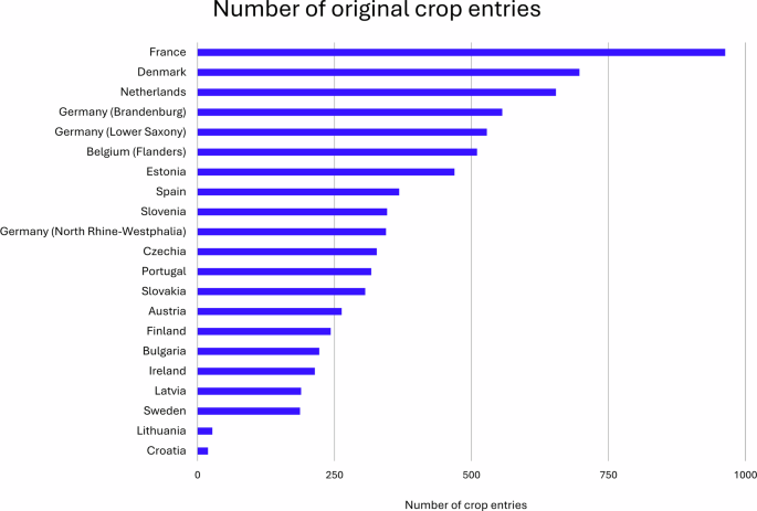
The number of different crop entries of the member states, federal states, and regions within our data inventory.
Pre-processing and harmonisation
To harmonise the datasets across all member states, we developed a uniform data structure of the spatial information and harmonised the information on crops and organic cultivation. The harmonisation was done separately for each member state, federal state, and region. Our harmonisation workflow included the following steps:
First, to explore the data and understand the meaning of data table columns, we listed all column names from the original vector data for each year, along with examples of the values stored in each column. This provided us with an understanding of the data structure and content. Additionally, we manually explored the data in QGIS.
To automate the subsequent steps, we created column-name lookup tables for each member state. This was necessary to automate the assignment of all the original columns to the harmonised column names (Table 2). The table included a separate column with the translation for each year, as column labels varied between years.
Table 2 Structure of the harmonised spatial data.
To harmonise the crops, we listed all available ‘crop code – crop name’ combinations in the vector data. In some cases, the meaning of the crop codes could change between years, or their descriptions could change. Working with the ‘crop code – crop name’ combinations ensured avoiding inconsistencies and misclassifications between the years. We then translated all crop names into English. In cases when a translation was not possible, we conducted a web search using the original crop entry.
For the harmonisation of the crop codes and crop names, we build on the proposed crop harmonisation of the EuroCrops project16. Therefore, when available, we used the crop-mapping tables from the EuroCrops project to categorise the ‘crop code – crop name’ combinations (https://github.com/maja601/EuroCrops/tree/main/csvs/country_mappings). In most cases, not all entries could be categorised automatically as the data include crops from multiple years, in contrast to EuroCrops. Hence, we manually expanded the existing EuroCrops tables and categorised all crops that had not been previously categorised. In cases where no crop-mapping table was available from EuroCrops, we manually categorised the crops. To reduce the workload, we used a string-matching algorithm on the English crop names, applying the Jaro-Winkler distance metric to associate unclassified entries with classified entries from other member states. The Jaro-Winkler metric measures string similarity based on the number of matching characters and transpositions (i.e., swapped letters). It is particularly useful for record matching and is therefore well-suited for matching crop type names19,20. All matching was performed on the English crop names. Manual verification of the matched entries and classification of any potentially remaining unclassified entries were still necessary; however, the workload was substantially reduced. Once the crop-mapping tables were finalised, we used them to harmonise the crop codes and names into the EuroCrops HCAT.
As described above, the EuroCrops HCAT consists of six hierarchical levels with increasing thematic details, but the original crop classifications of the member states provide different levels of detail. Sometimes, the crop codes of a member state fall into higher levels of the HCAT, while in other cases, they fall into lower levels. We extended the HCAT by including crop-mapping tables of nearly all EU member states (excluding Luxembourg and Malta) and by including historical data, in some cases going back to 2007, into our inventory. To facilitate interoperability with the EuroCrops database, we used the same column names as in the HCAT.
Across member states, there were differences in how the crop-specific information was stored in the data. In some member states, applicants can only declare a single crop at the parcel level, while in others, spatial data are only available at the reference-parcel level. Here, multiple crops can be declared within a reference parcel. When multiple crops were reported per reference parcel, our harmonised geospatial data only contain the crop information of one crop within the reference parcel. In such cases, the ‘field size’ refers to the entire reference-parcel area, while the ‘crop area’ refers to the area of the dominant crop reported in the crop columns. For example, if two crops are reported, with one crop covering 70% of the reference parcel and the other crop covering 30%, then the crop covering 70% is considered the dominant crop, and its area would be reported in the ‘crop area’ column. The additional crop data were saved in a complementary table linked to the reference parcel via the field ID.
Furthermore, we used the column-name translation tables to harmonise the column names. In most cases, the data included a unique national field ID. However, in cases where this ID was missing, we generated a running ID to ensure that all parcels have a unique identifier per member state. Where information was available, we extended the datasets by adding columns for farm identifiers or information on whether a parcel was managed organically. To harmonise the information on organic farming, we classified the parcels into three categories: ‘conventional’, ‘organic’, and ‘in conversion’ using the codes 0, 1, and 2, respectively. In some member states, this information was provided at the parcel level; in others, it was available only at the farm level. For the latter, we assigned the farm-level information to the respective parcels. Future versions of the harmonised inventory will include information on agri-environmental measures, eco-schemes, and animal numbers per farm. All geospatial data were transformed into a projected coordinate system (ETRS89-extended / LAEA Europe – EPSG:3035), and the files were saved as geoparquets.