Ethics
Experiments using transgenic Drosophila melanogaster stocks were approved under Chiba University Institutional Biosafety Committee protocol #G5-46.
Fly strains and keeping conditions
A cohort of 104 strains derived from the DGRP was used in our experiment. This panel consists of 205 inbred and genetically distinct strains of D. melanogaster, representing natural genetic diversity within a population captured in North Carolina, US. Flies were kept at 25 °C with about 40–60% humidity in a 12 L:12D cycle, with standard food (Bloomington Formulation, Nutri-Fly™, #66-113, Genesee Scientific). A visually defective mutant strain, w[*] norpA[P12] (BDSC#9047)62, was used to test the behavior of blind flies and the contribution of visual information in our assay. The following lines were used for functional assay of lamina neurons and Ptp99A: R9B08-GAL4 (w[1118]; P{y[+t7.7] w[+mC]=GMR9B08-GAL4}attP2/TM3, Sb[1]; BDSC#41369), Ptp99A-GAL4 (w[1118]; Mi{GFP[E.3xP3]=ET1}Ptp99A[MB04947]; BDSC#24843), UAS-TNT (w[*]; P{w[+mC]=UAS-TeTxLC.tnt}G2; BDSC#28838), UAS-IMPTNT (w[*]; P{w[+mC]=UAS-TeTxLC.(-)V}A2; BDSC#28840), UAS-Ptp99ARNAi (y[1] v[1]; P{y[+t7.7] v[+t1.8]=TRiP.JF01858}attP2; BDSC#25840). All fly strains were obtained from the Bloomington Drosophila Stock Center (BDSC), and the list of used strains with the stock number is summarized in Supplementary Data 7. Adult flies of both sexes aged at 2–4 days since eclosion were tested in the first behavioral screening with DGRP strains and norpA mutant (n = 20 per sex and social circumstance for each strain). Given the observed chasing behavior among male flies in several strains as described later, which likely impacts their social interaction, we used only female flies in a subsequent mixed-strain group experiment (n = 10 for each pair of strains) and mutant assay (n = 20 for each condition of strains).
To enable comparisons between the norpA mutant strain and DGRP strains, we backcrossed this mutant four times with DGRP208, a strain with intermediate behavioral phenotypes, while monitoring the norpA genotype using the following protocols. Genomic DNA was extracted from the whole body of a fly using the MightyPrep reagent (#9182, Takara Bio Inc., Japan) and amplified by PCR with MightyAmp DNA Polymerase (#R076A, Takara Bio Inc., Japan) and the primers targeting the mutated 240th residue63 (Table S1). The thermal cycling conditions were as follows: 98 °C for 1 min, followed by 30 cycles of 98 °C for 10 s, 59 °C for 15 s and 68 °C for 1 min. The amplified norpA cDNAs were digested with Cac8I (#R0579L, New England Biolabs Japan Inc., Japan) according to the manufacturer’s instructions, resulting in products of different lengths depending on the norpA genotype. During the backcrossing, we successfully eliminated the white mutation which can also affect the flies’ visual properties64, through recombination. This resulted in a strain that isolates the effect of the norpAP12 mutation in the DGRP208 genetic background. The confirmed sequences of norpA and eye phenotypes are shown in Fig. S19.
Behavioral assay under looming stimuli
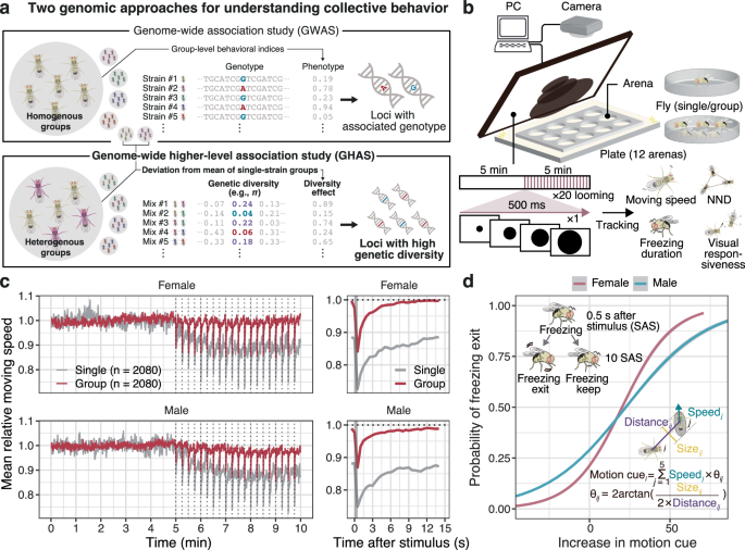
Behavioral assays were conducted as previously described65. Briefly, flies were tested individually or in single-sex groups (n = 6) to avoid sexual behavior that could confound threat responses. We chose six individuals to be grouped since the previous study demonstrated the number to be enough to show group effect in the assay26. Flies were placed in arenas with sloped walls (30 mm in diameter, 2 mm deep), and looming stimuli were presented on a 13.3-inch monitor tilted 45° toward the plate, as detailed in our previous study65. The flies’ behavior was recorded at approximately 50 frames per second using a USB3 camera (DMK33UX290, The Imaging Source, Germany) controlled by a custom python script. Recorded videos were trimmed per arena and tracked using Tracktor software66, followed by additional error corrections with custom scripts65. To further reduce the calibration errors of tracking, the weighted moving average of coordinates over a time span (9 preceding time points including a time point of interest) was used for analysis. The coordinates were subsequently used to calculate the distance traveled from a previous time point, moving speed (traveled distance divided by frame intervals), and head angle (calculated by the movement between time points 50 ahead and behind the time point of interest) for each time point. These measures were averaged at 0.5-s intervals and used for subsequent analyses. Locomotor behavior was briefly dichotomized as walking when their speed was > 4 mm/s or stopping otherwise25. Freezing was defined when a fly that stopped 0.5 s after a stimulus continued to stop 10 s after the stimulus, otherwise referred to as freezing exit.
Calculation and analysis of behavioral indices
The average moving speed during the first 5 min with no stimuli was assessed to be an index of baseline locomotor activity. To quantify the level of the sociality of flies, we calculated the NND at a time point when all the flies in a given arena were expected to be at rest (i.e., a time point when the average moving speed across flies were minimum during the 5 min). For comparison, pseudo-group data consisting of random combinations of single fly data were created and evaluated as a control with no social preference. In this process, an experimental date, time, and used plate and arena was randomly chosen from the information of constituting flies and used as covariates for the data. In the latter 5 min of the experiment, the average time taken to restore the moving speed to the baseline level (i.e., the mean moving speed during the first 5 min) after exposure to stimuli was used as an indicator of the fear response to threatening stimuli. In order to quantify the flies’ response toward other individuals, we first calculated the “motion cue” that each fly is expected to perceive from other flies for each time step, defined as follows (Fig. 1d; modified from ref. 26):
$${M}_{i}=\mathop{\sum }\limits_{j=1}^{5}{V}_{j}{\theta }_{{ij}}$$
(1)
$${\theta }_{{ij}}=\,2\arctan \left(\frac{{{size}}_{{ij}}}{2\,{{distance}}_{{ij}}}\right)$$
(2)
where for a focal fly i in a group, the motion cue it perceived (\({M}_{i}\)) was defined as the sum of other flies’ speed multiplied by the visual angle. \({V}_{j}\) and \({\theta }_{{ij}}\) represent the moving speed and the visual angle of the individual j on the retina of the individual i, respectively. The distance between individuals i and j (\({{distance}}_{{ij}}\)) was calculated from their centroids, and the visual size of the individual j to i (\({{size}}_{{ij}}\)) was calculated by projecting the individual j’s body (represented by an ellipse with 1 and 2 mm in a smaller and larger radius, respectively) on the body axis of the individual i as described in Fig. 1d. Next, we modeled the probability of freezing exit (\({P}_{{{\rm{FE}}}}\)) explained by the increase in perceived motion cues in 10 s after a stimulus with a following logistic regression:
$${P}_{{{\rm{FE}}}}=\frac{1}{1+{e}^{-({\beta }_{0}+{\beta }_{1}x)}}$$
(3)
Here, the intercept β0 was used as an index of response threshold, representing flies’ visual responsiveness toward motion cues of other conspecifics. To accurately estimate the logistic curve fitting to the visual response of each strain of flies, we pooled the data of all stimulating trials (6 individuals × 20 trials × 20 replicates = 2400 data points at maximum) and conducted above regression for each strain. In case for the dataset of GAL4/UAS strains, we randomly sampled 500 data points from all the dataset of a given strain to perform logistic regression and repeated it for 20 times to obtain the β0 estimates for the population. Considering that the primary focus of this study is on the responsiveness to conspecifics, we further quantified this by introducing an additional metric: the mean cumulated motion cues each individual received on freezing exit (defined as moving speed > 4 mm/s). We then sought to identify genetic variants associated with this metric. The results similarly indicated genetic involvement of nervous system (Fig. S20 and Supplementary Data 8). Thus, given the high correlation between males and females, we decided to use the previously mentioned metric (β0) as the main result.
Given the significant observation of male chasing behavior across several strains, we quantified both the duration of chasing and chaining behavior (involving three or more individuals in a chain) within the initial 5 min of experiment. Chasing is defined based on three criteria: (1) both individuals must be moving at a speed greater than 1 mm/s; (2) their orientations must be aligned within an angular difference of π/4; and (3) the distance between them must be less than 3 mm. Chaining behavior occurs when these chasing interactions form a sequence, such that individual A chases B, and B chases C, establishing a continuous chain of chases.
Behavioral simulation with individual-based model
To explore the mechanisms behind the observed changes in fear responses in fly groups and the diversity effect in mixed-strain groups, we conducted behavioral simulations using an IBM (Fig. S6a). The arena size was set to 30 mm, and the number of agents in the arena was set to one in the single condition and six in the group and mixed-strain group conditions. Like the actual experiments, each time step was set to 0.02 s, replicating a 10-min experiment (i.e., 30,000 frames in total). The moving speed of the agent at time t (\({V}_{t}\)) followed a Lévy distribution with a mean speed of 3.8 mm/s, obtained from our experimental data, and a shape parameter α = 2, with a change in moving direction (\({D}_{t}\)) following a normal distribution with a mean of 0 and a standard deviation of π:
$${V}_{t} \sim {{\rm{L}}} {\acute{{\rm{e}}}} {{\rm{vy}}}(\mu=3.8\,{{\rm{mm}}}/{{\rm{s}}},\alpha=2)$$
(4)
$${D}_{t} \sim {{\rm{Normal}}}(0,\pi )$$
(5)
The Lévy distribution was chosen to simulate the natural movement patterns observed in biological organisms. Let the vector representing the agent’s heading direction be \({\mathbb{v}}\), and the normal vector to the nearest wall from the agent’s current position be \({\mathbb{n}}\). The angle between these two vectors, representing agent’s angle to wall, can be calculated as follows:
$$\theta={{\rm{atan}}}2\,({\mathbb{v}}{\mathbb{\times }}{\mathbb{n}}{\mathbb{,}}{\mathbb{v}}\cdot {\mathbb{n}})$$
(6)
where \({\mathbb{v}}{\mathbb{\times }}{\mathbb{n}}\) represents the z component of cross product of \({\mathbb{v}}\) and \({\mathbb{n}}\), calculated as \({v}_{x}{n}_{y}-{v}_{y}{n}_{x}\), and \({\mathbb{v}}{\mathbb{\cdot }}{\mathbb{n}}\) represents the dot product of the two vectors. If the agent approaches the wall, it decelerates its moving speed in 50% and changes the direction to avoid wall. The updated moving speed (\({V}_{t}^{\prime}\)) and direction (\({D}_{t}^{\prime}\)) at time t are defined as follows:
$${V}_{t}{\prime}=\left\{\begin{array}{c}0.5{V}_{t} \quad {{\rm{if}}}\; {{\rm{distance}}}\; {{\rm{to}}}\; {{\rm{wall}}}
(7)
$${D}_{t}^{\prime} \sim {{\rm{Normal}}}\left({{\rm{sign}}}(\theta )\left(\frac{\pi }{2}-\left|\theta \right|\right),\frac{\pi }{18}\right)$$
(8)
To introduce a temporal correlation in movement speed, we further incorporated a speed inheritance mechanism in the model. The speed at time t (\({V}_{t}\)) is calculated as a weighted sum of 60% of the speed from the previous timestep (\({V}_{t-1}\)) and 40% of the current adjusted speed (\({V}_{t}^{\prime}\)):
$${V}_{t}=0.6{V}_{t-1}+0.4{V}_{t}^{\prime}$$
(9)
Next, visual stimuli were introduced every 15 s starting 5 min into the experiment, defined by a fixed probability of stopping movement. Immediately after a stimulus is given at time t, there’s a 90% chance that the moving speed becomes 0. This state is represented by \({S}_{t}\), where \({S}_{t}=1\) if the moving speed becomes 0, and \({S}_{t}=0\) otherwise.
$${S}_{t}=\left\{\begin{array}{cc}1 & {{\rm{with}}}\; {{\rm{probability}}}\,0.9\\ 0 & {{\rm{otherwise}}}\hfill\end{array}\right.$$
(10)
$${V}_{t}=\left\{\begin{array}{cc}0 &\!\!\!\!\!\!{{\rm{if}}}\,{S}_{t}=1\\ {V}_{t} & {{\rm{otherwise}}}\end{array}\right.$$
(11)
If the moving speed becomes 0 immediately after a stimulus (\({S}_{t}=1\)), the subsequent moving speed for up to 15 s until the next stimulus follows a probability function as below, where a and b are constants, and t’ is the time elapsed after the stimulus, up to 15 s.
$${{\rm{For}}}\,{t}^{{\prime} }{{\rm{seconds\; after}}}\,{S}_{t}=1\,{{\rm{where}}}\,0\,
$$P\left({V}_{t+{t}^{{\prime} }}=0\left|{S}_{t}=1\right.\right)=\max (0,1-(a\log \left({t}^{{\prime} }\right)+b))$$
(12)
The relationship and values of parameters \(a\) and \(b\) used in the log function were determined based on actual fly data. Specifically, we fitted a log function (\(y=a\log \left(x\right)+b\)) to velocity data normalized by the average at 0.5 s before looming stimuli (Fig. S7a), and from this fitting derived the regression equation \(b=1.02-2.45a\) (Fig. S7b). Considering the observed range of the empirical data, we applied \(a\) = 0.02 into the model for single-strain conditions and used \(a\) = [0.005, 0.006, 0.007, 0.008, 0.009, 0.01, 0.02, 0.03, 0.04, 0.05, 0.06, 0.07, 0.08, 0.09, 0.1] to represent 15 distinct strains differing in the extent of freezing, and conducted simulations of mixed-strain groups under these parameter settings. Lastly, we incorporated the change in motion cues of other individuals from time \(t-2\) to \(t-1\) into individual’s moving speed at time \(t\), thereby updating their speed based on social interaction.
$${V}_{t}=(1-s){V}_{t}+s({M}_{t-1}-{M}_{t-2})$$
(13)
where \({M}_{t-1}{-M}_{t-2}\) represent the change in motion cues between previous time steps, and social factor \(s\) refers to the proportion of motion cues incorporated to adjust individual’s speed to others. We have set this parameter in two patterns: \(s=0.1\) and \(s=0\) for agents with and without speed alignment mechanism, respectively.
Additionally, to validate the suitability of these three parameters related to freezing and synchronization in movement, we performed a grid search for the parameters \(a\), \(k\), and \(s\) under the constraint \(b=1-{ka}\), thereby exploring parameter sets that best matched the actual behavioral patterns of the flies (Fig. S8). The discrepancy between simulated and real data were calculated for each condition based on the time-series normalized velocity data described above.
Statistical analysis for behavioral traits
Statistical analysis of behavioral data was performed using R 4.4.2 with the car, lmerTest, and lme4 packages when necessary. Effects of strains, sex, social circumstances, and their interactions on behavioral measures were assessed with the linear mixed model (LMM) with experimental date, time, used plate and arena assumed to be random effects. To assess the significance of fixed effects in the LMM, we applied a Type II Wald chi-square test. The broad-sense heritability of traits was estimated by the formula described in previous studies67,68 using mean squares for genotype (strain) and environment (residual error) obtained in analysis from variance (ANOVA). The results of ANOVA are shown in Table S2.
Genome-wide association analysis
We first performed principal component analysis (PCA) to capture the genetic distance among strains, using a whole set of genotypes of 4,438,427 SNPs for 205 strains obtained from the DGRP2 website (http://dgrp2.gnets.ncsu.edu) with PLINK v1.969. Quality control of SNPs was carried out with conditions: (1) minor allele frequency >0.05 and (2) SNP call rate > 0.9, leaving 1,689,110 SNPs for subsequent analyses. Prior to GWAA, SNP-based heritability and genetic correlation among phenotypes were estimated by SCORE70. We then performed GWAA to identify loci responsible for the three phenotypes (i.e., freezing duration, NND, and visual responsiveness) of flies. The behavioral phenotypes were regressed with the top 10 PCs as covariates using GCTA v1.94.0 with –fastGWA-mlm flag71, based on a linear mixed model and a SNP-derived sparse genetic relationship matrix. The association analysis was performed independently for each sex, and loci with the P-values below the genome-wide significance level as P = 1.0 × 10⁻⁵ were detected to be candidates associated with the given phenotype. For visual responsiveness metrics, we have performed a meta-analysis of the GWAS results from both sexes using METAL72, and genome-wide significance level was set to P = 1.0 × 10⁻⁶. GO enrichment analysis for candidate loci was conducted independently for both sexes using the clusterProfiler package in R.
Single-cell transcriptomic analysis of Drosophila visual neurons
Single-cell RNA-seq dataset of the developing visual neurons of D. melanogaster53 was reanalyzed. The dataset included expression data of visual neurons from female offspring of W1118 crossed with various DGRP strains across nine developmental stages (0–96 h APF). Due to differences in tissue composition and coverage53, we used the main dataset comprising 24–96 h APF. Each cell was annotated based on the previous study53, and cell clusters were visualized using t-distributed stochastic neighbor embedding (t-SNE). We specifically focused on motion-detecting neurons54, including R1/6, L1–5, Tm1–4, 9, and T4/5 cells. To compared the expression levels of Ptp99A between the genotypes (C and T alleles of 3 R:25292746) detected in GWAS, we used generalized linear mixed model with a gamma distribution, treating strains and replications as random effects, implemented with the glmer() function from the lme4 package in R. Finally, we conducted weighted gene coexpression network analysis (WGCNA) using the hdWGCNA package73 in R. The 2,000 most variably expressed genes across the above neurons were selected for analysis, resulting in five major coexpression modules. Eigengene expression levels for each module were compared between the Ptp99A genotypes using Wilcoxon’s rank sum test.
Mixed-strain group experiments and calculation of diversity effect
Among the 104 strains used in GWAS, we selected genomically diverse 15 strains (cf., Fig. S7a) and prepared groups of 6 female flies, composed of 3 individuals from each of the two different strains (i.e., 105 pairs of strain in total; n = 10 for each). Following the behavioral experiment, the average moving speed among individuals relative to that of first 5 min in a mixed-strain group was compared with the average values of the two strains that constitute the group. Subsequently, visual stimuli were considered as hypothetical predators, and virtual behavioral performance was defined based on the flexible behavioral changes observed in response to the stimuli. Assuming that freezing under predatory pressure and exploration in its absence are adaptive strategies, we calculated a weighted sum of moving speed, assigning a negative coefficient to the freezing term and a positive coefficient to the exploration term (Fig. 4a). Given that flies’ moving speed typically returned to baseline within 3 seconds after a visual stimulus and based on subsequent experiments with predatory spiders, the freezing term was defined as 0–2.5 seconds after stimulus, and the exploration term as 3–14 seconds after stimulus. Weights were applied to account for the differing durations of these time periods in the calculation (Fig. 4a). The difference between the observed performance level of mixed-strain groups and the expected performance level (calculated as the average values of single-strain groups for the two strains) was defined as the diversity effect (Fig. S14).
Animal-computer interaction experiments with predatory spiders
To explore the adaptive significance of behavioral switching from freezing to exploration, we conducted an animal-computer interaction experiment using jumping spiders (Hasarius adansoni), a well-known predator of fruit flies27,28. A total of 20 trials were conducted with 14 wild-caught male spiders, starved for over 5 days, each placed in a Petri dish (84 mm diameter, 1.5 cm height) on a screen displaying a virtual fly. A black ellipse, 2 mm in length, was used to mimic a fly as it is simple enough to attract jumping spiders74. The experiment was performed under the same environmental condition as previous fly experiments, with the spider’s position tracked for 5 min using the same camera and a custom python script, yielding 1200 frames of data per trial (summarized into 0.25-s bins). The virtual flies’ movement followed a Lévy distribution with α = 1.5, with mean speeds set at three levels: slow ( ~2.5 mm/s), medium ( ~5.0 mm/s), and fast ( ~7.5 mm/s). To simulate the fly’s freezing response, its movement stopped for specified durations (0, 1, 3, 6, or 12 s) when the tracked spider approached within a proximity range (1 or 2 cm). Each spider was sequentially exposed to all conditions, with the order of presentation randomized to minimize potential bias. To prevent perpetual inactivity caused by a stationary spider, the virtual fly resumed movement for 3 seconds after each freezing period. A spider attack was defined as an instance where spider’s moving speed exceeded 30 mm/s and approached within 1 cm of the virtual fly in 3 consecutive frames. Given the spider’s strong attraction to the virtual fly at the highest speed tested (7.5 mm/s) and the shorter proximity range (1 cm) (Fig. S13a), these conditions were selected for the main analysis. Trials in which the spider attacked less than once on average across all freezing conditions were excluded from the analysis. Spider ID, trial, and experimental order (Fig. S13b) were included as random effects in LMM.
To further evaluate the behavioral performance of fly groups, we conducted an additional experiment using six agents in the arena with the same environmental and feeding conditions. In this experiment, we employed the same locomotion speed (7.5 mm/s) and proximity range (1 cm) as described above. Freezing durations were set to 1, 3, 6, and 12 s, and we recreated mixed-strain fly groups by combining agents with different freezing durations (three agents of one value and three of another). We also varied whether or not alignment in moving speed occurred among the agents, resulting in 20 distinct movement conditions. As the above single-agent experiment, each virtual fly group was then exposed to a spider for five minutes in a random order, and we assessed their behavioral performance based on a principal component score integrating the longer distance traveled by the flies and the fewer number of spider attacks, corrected by the order of experiment. A total of 10 individual spiders were used, each tested twice in this grouped-fly experiment. For seven of these spiders (m1–5, m15, and m16 in Fig. S17a), only the 3- or 6-s freezing durations were used in the first trial, meaning the number of experimental conditions for those spiders differed from that of the others.
Identifying responsible loci for diversity effect with GHAS
The diversity effect was computed per combination of strains and may be explained by the genetic differences (diversity) between the two strains. To comprehensively explore the responsible loci for the diversity effect, we calculated the nucleotide diversity (π) at each locus (1000 bp windows) from the genome sequences of the two strains constituting the mixed group using vcftools75 and conducted an association analysis with the diversity effect, which we termed the GHAS. Genetic relatedness matrix of the analyzed strains was used as covariates. The same threshold as the above GWAA (P –5) was applied to determine candidate loci, and GO enrichment analysis on the adjacently located genes ( ± 1 kbp) was performed using the R package clusterProfiler.
Reporting summary
Further information on research design is available in the Nature Portfolio Reporting Summary linked to this article.