Meson form factors
Pion has two GFFs which are defined as18,20,59,60,61
$$ \left\langle {\pi }^{a}({p}^{{\prime} })\left\vert {\hat{T}}^{\mu \nu }\right\vert {\pi }^{b}(p)\right\rangle \\ \;\;=\frac{{\delta }^{ab}}{2}\left[{A}^{\pi }(t){P}^{\mu }{P}^{\nu }+{D}^{\pi }(t)\left({\Delta }^{\mu }{\Delta }^{\nu }-{g}^{\mu \nu }{\Delta }^{2}\right)\right],$$
(3)
where a, b = 1, 2, 3 are isospin labels. We work in the isospin limit. Elastic unitarity gives the imaginary part from ππ intermediate states via the Cutkosky cutting rule62 (see Fig. 1),
$$\,{{\mbox{Im}}}\,{A}^{\pi }(t)={\sigma }_{\pi }(t){\left({t}_{2}^{0}(t)\right)}^{*}{A}^{\pi }(t),$$
(4)
$$\,{{\mbox{Im}}}\,{D}^{\pi }(t)=\, {\sigma }_{\pi }(t)\left[\frac{1}{3}{\sigma }_{\pi }^{2}(t){\left({t}_{0}^{0}(t)-{t}_{2}^{0}(t)\right)}^{*}{A}^{\pi }(t)\right. \\ \left.+{\left({t}_{0}^{0}(t)\right)}^{*}{D}^{\pi }(t)\right],$$
(5)
where \({\sigma }_{i}(t)\equiv \sqrt{1-4{m}_{i}^{2}/t}\) (i = π, K and N) and \({t}_{0}^{0}(t)\) (\({t}_{2}^{0}(t)\)) are the S-(D-)wave ππ partial-wave amplitudes related to the phase shifts \({\delta }_{\ell }^{0}(t)\) according to \({t}_{\ell }^{0}(t)={e}^{i{\delta }_{\ell }^{0}(t)}\sin {\delta }_{\ell }^{0}(t)/{\sigma }_{\pi }(t)\). Details of the derivation of Eqs. (4) and (5) are given in the Supplementary Material. In practice, the phase of the ππ D-wave scattering amplitude \({\phi }_{2}^{0}(t)\) instead of \({\delta }_{2}^{0}(t)\) is used to include inelastic effects. The D-wave data are taken from the latest crossing-symmetric dispersive analysis63 instead of ref. 64 used in ref. 65. The main difference lies in the fact that the phase shift and inelasticity from ref. 63 are consistent with the commonly used results64 below 1.4 GeV and cover a larger energy range up to around 2 GeV. The difference turns out to be moderate.
Fig. 1: Elastic unitarity relation for the pion GFFs Fπ = {Aπ, Dπ}.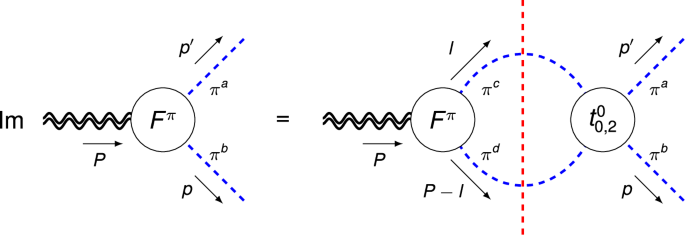
The blue dashed lines denote pions, the double wiggly lines represent the external QCD EMT current, and the red vertical dashed line indicates that the intermediate pion pair are to be taken on-shell.
One sees from Eq. (4) that the phase of the GFF Aπ equals \({\delta }_{2}^{0}\) (or \({\phi }_{2}^{0}\), modulo multiple of π). The dispersion relation admits a solution known as the Omnès representation66:
$${A}^{\pi }(t)=(1+\alpha t){\Omega }_{2}^{0}(t),$$
(6)
$${\Omega }_{2}^{0}(t)\equiv \exp \left\{\frac{t}{\pi }\int_{4{m}_{\pi }^{2}}^{\infty }\frac{{{\rm{d}}}{t}^{{\prime} }}{{t}^{{\prime} }}\frac{{\phi }_{2}^{0}({t}^{{\prime} })}{{t}^{{\prime} }-t}\right\}.$$
(7)
The coefficient α can be estimated using the NLO ChPT result with a tensor meson dominance estimate for the relevant low-energy constant (LEC) \({L}_{12}^{r}\)59. Namely, \(\alpha=-2{L}_{12}^{r}/{F}_{\pi }^{2}-{\dot{\Omega }}_{2}^{0}(0)\) and \({L}_{12}^{r}=-{F}_{\pi }^{2}/(2{m}_{{f}_{2}}^{2})\), where Fπ = 92.1MeV is the physical pion decay constant, \({m}_{{f}_{2}}=(1275\pm 20)\,\)MeV is the mass of the f2(1270) resonance, with the uncertainty covering various experimental measurements67 for a conservative estimate, and the dot notation indicates the derivative with respect to t.
However, Eq. (5) is notably more complicated because the GFF Dπ mixes the JPC = 0++ and 2++ quantum numbers, where J is angular momentum (AM) and P, C are parity and charge conjugation, respectively. We can define the pion trace GFF68,69, \({\Theta }^{\pi }(t)=-t\left[{\sigma }_{\pi }^{2}(t){A}^{\pi }(t)+3{D}^{\pi }(t)\right]/2\). Then Eq. (5) leads to a standard single-channel partial-wave unitarity relation \(\,{\mbox{Im}}\,{\Theta }^{\pi }(t)={\sigma }_{\pi }(t){\left({t}_{0}^{0}(t)\right)}^{*}{\Theta }^{\pi }(t)\), in analogy to Eq. (4).
To account for the strong ππ-\(K\bar{K}\) interactions in the 0++ channel due to the f0(980) resonance, we consider the coupled-channel Muskhelishvili-Omnès problem66,70, given as71
$$\,{\mbox{Im}}\,{{\mathbf{\Theta }}}(t)={[{{{\bf{T}}}}_{0}^{0}(t)]}^{*}{{{\mathbf{\Sigma }}}}_{0}^{0}(t){{\mathbf{\Theta }}}(t),$$
(8)
where \({{\mathbf{\Theta }}}(t)={\left({\Theta }^{\pi }(t),2{\Theta }^{K}(t)/\sqrt{3}\right)}^{T}\), and the definitions of T-matrix \({{{\bf{T}}}}_{0}^{0}(t)\) and phase-space factor \({{{\mathbf{\Sigma }}}}_{0}^{0}(t)\) can be found in refs. 71,72 (see also Supplementary Eqs. (27) and (29)). Using Eq. (8), the trace FFs can be written as71
$${\left(\begin{array}{c}{\Theta }^{\pi }(t)\\ \frac{2}{\sqrt{3}}{\Theta }^{K}(t)\end{array}\right)}^{T}={\left(\begin{array}{c}2{m}_{\pi }^{2}+{\beta }_{\pi }t\\ \frac{2}{\sqrt{3}}\left(2{m}_{K}^{2}+{\beta }_{K}t\right)\end{array}\right)}^{T}{{{\mathbf{\Omega }}}}_{0}^{0}(t),$$
(9)
by virtue of the S-wave Omnès matrix \({{{\mathbf{\Omega }}}}_{0}^{0}\)72. Notice that the parameters βπ and βK cannot be zero due to chiral symmetry71, and their values are related to the slopes of GFFs at t = 0, i.e., \({\dot{\Theta }}^{\pi }(0)=0.98(2),{\dot{\Theta }}^{K}(0)=0.94(14)\), matching to the prediction of ChPT at NLO59. The uncertainties from higher order chiral corrections are much smaller than the above quoted errors and thus negligible. We refer to the Supplementary Material for further details.
We use precise phase shifts and inelasticities from analyses in refs. 63, 73, 74 as inputs. The predictions for the pion GFFs are shown in Fig. 2, where the uncertainties are obtained from the variations in \({m}_{{f}_{2}}\) and the slopes \({\dot{\Theta }}^{\pi }(0)\) and \({\dot{\Theta }}^{K}(0)\) mentioned above (prediction of the kaon trace GFF ΘK is shown in Supplementary Fig. 4). We have checked that errors caused by those of the D-wave phase and the S-wave Omnès matrix are negligible. That is, the uncertainties are from the low-energy inputs from matching the dispersion representation of the meson GFFs to the NLO ChPT expressions, and can be further reduced once the involved LECs are precisely determined from lattice QCD calculations. Our results agree well with LQCD calculations at an unphysical pion mass of 170 MeV75.
Fig. 2: The total GFFs Aπ, Θπ and Dπ of the pion.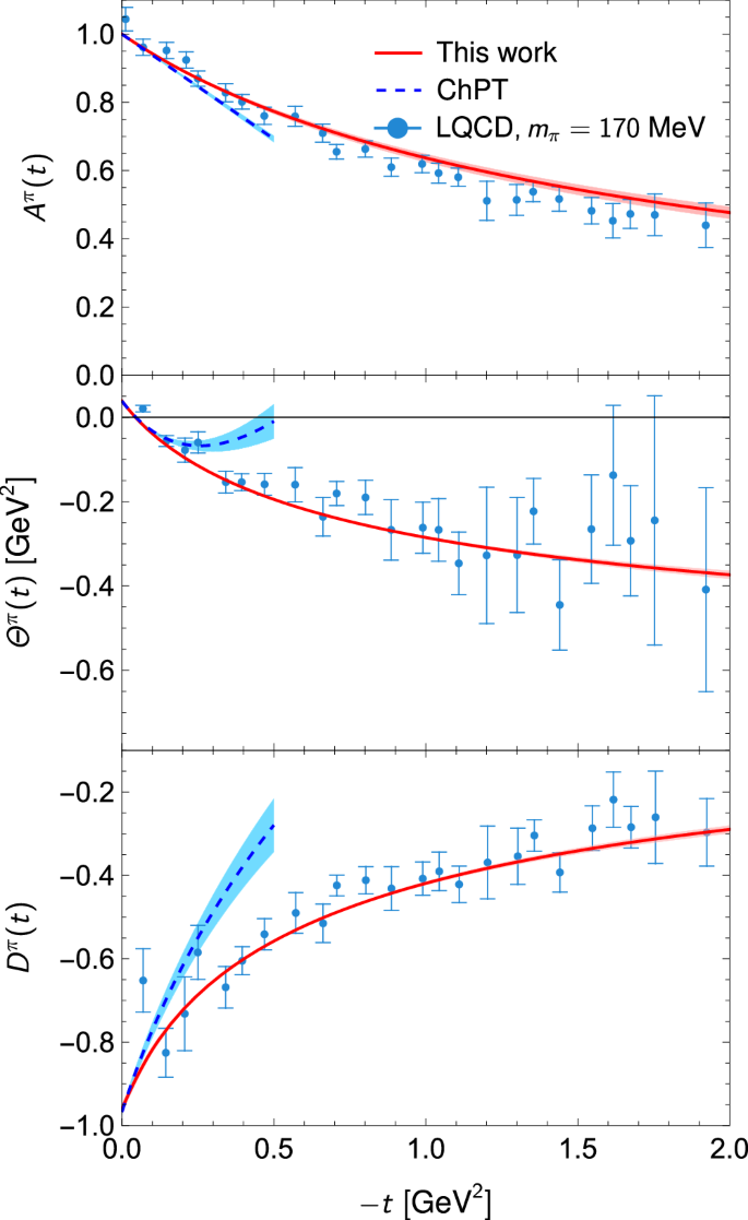
Our predictions are shown as red solid lines. The blue dashed lines show the NLO ChPT prediction for the low − t region59. We also show the LQCD results at mπ = 170 MeV for Aπ and Dπ in ref. 75; Θπ is obtained from a linear combination of Aπ and Dπ, with errors added in quadrature.
We note that the study of pion GFFs using the dispersion approach was pioneered in ref. 71 with low-precision data, and further developed for Θπ recently in ref. 69 by incorporating S-wave ππ-\(K\bar{K}\) scattering from dispersive analysis in ref. 8 and fitting lattice data75. We advance the dispersive analysis in both Θπ and Aπ GFFs by utilizing precise phase shifts63,73 and NLO ChPT results59, achieving theoretical predictions without the need for lattice data fitting.
Nucleon form factors
The above dispersive treatment can be generalized to the nucleon case, for which the unitarity relation is depicted in Fig. 3. Following the notation of refs. 76,77,78, we have
$$\,{{\mbox{Im}}}\,A(t)=\frac{3{t}^{2}{\sigma }_{\pi }^{5}}{32\sqrt{6}}{\left[{f}_{-}^{2}(t)+\frac{2\sqrt{6}{m}_{N}}{t{\sigma }_{N}^{2}}{\Gamma }^{2}(t)\right]}^{*}{A}^{\pi }(t),$$
(10)
$$\,{{\mbox{Im}}}\,J(t)=\frac{3{t}^{2}{\sigma }_{\pi }^{5}}{64\sqrt{6}}{\left({f}_{-}^{2}(t)\right)}^{*}{A}^{\pi }(t),$$
(11)
$$\,{{\mbox{Im}}}\,D(t)=\, -\frac{3{m}_{N}{\sigma }_{\pi }}{t{\sigma }_{N}^{2}}\left[\frac{{\sigma }_{\pi }^{2}}{3}{\left({f}_{+}^{0}(t)-{\left(\frac{t{\sigma }_{\pi }{\sigma }_{N}}{4}\right)}^{2}{f}_{+}^{2}(t)\right)}^{*}\right.\\ \times \left.{A}^{\pi }(t)+{\left({f}_{+}^{0}(t)\right)}^{*}{D}^{\pi }(t)\right],$$
(12)
where \({f}_{+}^{0}(t)\) and \({f}_{\pm }^{2}(t)\) are the S- and D-wave amplitudes for \(\pi \pi \to N\bar{N}\), and \({\Gamma }^{2}(t)\equiv {m}_{N}\sqrt{2}{f}_{-}^{2}(t)/\sqrt{3}-{f}_{+}^{2}(t)\). A detailed derivation of these equations can be found in the Supplementary Material.
Fig. 3: Elastic unitarity relation for the isoscalar nucleon GFFs FN = {A, J, D}.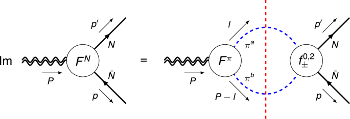
The blue dashed, black solid, and double-wiggly lines denote pions, nucleons, and the external QCD EMT current, respectively; the red dashed vertical line indicates that the intermediate state ππ are to be taken on-shell.
Using Eqs. (10), (11) and Eq. (12), the explicit formula of the spectral function ImΘ can be written as79
$$\,{{\rm{Im}}}\,\Theta (t)=-\frac{3{\sigma }_{\pi }}{2t{\sigma }_{N}^{2}}{\left({f}_{+}^{0}(t)\right)}^{*}{\Theta }^{\pi }(t).$$
(13)
It can also be generalized to include \(K\bar{K}\) intermediate states,
$$\,{{\rm{Im}}}\,\Theta (t)=\, -\frac{3}{2t{\sigma }_{N}^{2}}\left[{\sigma }_{\pi }{\left({f}_{+}^{0}(t)\right)}^{*}{\Theta }^{\pi }(t)\theta (t-4{m}_{\pi }^{2})\right.\\ +\left.\frac{4}{3}{\sigma }_{K}{\left({h}_{+}^{0}(t)\right)}^{*}{\Theta }^{K}(t)\theta (t-4{m}_{K}^{2})\right],$$
(14)
where \({h}_{+}^{0}\) is the S-wave amplitude for \(K\bar{K}\to N\bar{N}\). The channel \(K\bar{K}\) is important because the scalar resonance f0(980) strongly couples to \(K\bar{K}\) and also to ππ.
Once the spectral functions of nucleon GFFs are obtained from the Omnès representation of the meson GFFs in Eqs. (6), (9) and the \(\pi \pi /K\bar{K}\to N\bar{N}\) partial wave amplitudes, the nucleon GFFs can be constructed from the spectral functions, by the unsubtracted dispersion relations (DRs),
$$(A,J,\Theta )(t)=\frac{1}{\pi }\mathop{\int}\nolimits_{4{m}_{\pi }^{2}}^{\infty }{{\rm{d}}}{t}^{{\prime} }\frac{\,{{\mbox{Im}}}\,(A,J,\Theta )({t}^{{\prime} })}{{t}^{{\prime} }-t},$$
(15)
whose convergence is ensured by the leading order perturbative QCD analyses80,81,82.
One immediately obtains sum rules for the normalization of the nucleon GFFs,
$$\frac{1}{\pi }\mathop{\int}\nolimits_{4{m}_{\pi }^{2}}^{\infty }{{\rm{d}}}{t}^{{\prime} }\frac{\,{{\mbox{Im}}}\,(A,J,\Theta )({t}^{{\prime} })}{{t}^{{\prime} }}=\left(1,\frac{1}{2},{m}_{N}\right),$$
(16)
and, using Eq. (2), D-term satisfies the following sum rule:
$$D(0)=\frac{4{m}_{N}}{3\pi }\mathop{\int}\nolimits_{4{m}_{\pi }^{2}}^{\infty }{{\rm{d}}}{t}^{{\prime} }\frac{\,{{\mbox{Im}}}\,\left({m}_{N}A({t}^{{\prime} })-\Theta ({t}^{{\prime} })\right)}{{t}^{{\prime} 2}}\,.$$
(17)
The sum rules in Eq. (16) serve as a strong constraint so that any violation implies breaking of the Poincaré symmetry. In fact, if the spectral functions are rigorously known, these sum rules will be satisfied. However, the integrals on the left-hand side of Eq. (16) do not always converge sufficiently fast to fully satisfy the sum rules, as also found before in the dispersive analysis of the nucleon electromagnetic form factors. To address this, following refs. 83,84,85,86, we introduce additional effective zero-width poles with masses mS,D into the spectral functions (10), (11) (D-wave) and (14) (S-wave), represented as \(\pi {c}_{S,D}{m}_{S,D}^{2}\delta \left(t-{m}_{S,D}^{2}\right)\), to simulate contributions from highly excited meson resonances. One effective pole is introduced for each partial wave, and the S- and D-wave couplings cS,D are fixed to ensure the sum rules (16) align with their expected values. The poles correspond to the highly excited meson resonances above ~1.4 GeV (up to about this energy the phases are precisely known) contributing to the spectral function. Their contributions are minor in the low ∣t∣ region for the GFFs, and we vary the pole locations to estimate the high energy uncertainty.
Equations (10), (11), (14), and (15) are the master formulae used to compute the nucleon GFFs. The input \(\pi \pi /K\bar{K}\to N\bar{N}\,S\)-wave amplitudes are from the rigorous Roy-Steiner equation analyses65,72,79,87,88. In particular, we take the ones from ref. 88 (see Supplementary Fig. 6). This method imposes general constraints on πN scattering amplitudes, such as analyticity, unitarity, and crossing symmetry. The partial waves for \(\pi \pi \to N\bar{N}\) are incorporated into a fully crossing-symmetric dispersive analysis, ensuring that the spectral function complies with all analytic S-matrix theory requirements and low-energy data constraints. The ππ-\(K\bar{K}\) two-channel approximation works very well up to about 1.3 GeV, beyond which inelasticities due to the 4π channels start to play a role. It is important to note that two subtractions were implemented in the πN Roy-Steiner equation analysis, which significantly suppress contributions from the high-energy region72. The remaining high-energy contributions are accounted for by the aforementioned effective poles. This approach has been successfully applied to nucleon scalar form factors72, the πN σ-term89,90,91, electromagnetic form factors84,86, and antisymmetric tensor form factors92. For the D-wave contributions in Eq. (10) and Eq. (11), we adopt the results from ref. 63, which differ slightly from those in ref. 65, as noted above.
The uncertainties of our results come from three sources: (i) uncertainties of the LECs in NLO ChPT59, which are obtained by varying α ∈ [ − 0.03, 0.01] GeV−2, βπ ∈ [0.68, 0.72] and βK ∈ [0.32, 0.60], corresponding to varying \({L}_{12}^{r}\), \({\dot{\Theta }}^{\pi }(0)\) and \({\dot{\Theta }}^{K}(0)\) as given above in the mesonic sector; (ii) uncertainties of the \(\pi \pi /K\bar{K}\to N\bar{N}\) partial wave amplitudes, which have been fully estimated in the comprehensive review of the πN Roy-Steiner equation analysis65; (iii) uncertainties of the high-energy tail of the spectral functions, estimated by varying the effective pole masses. In practice, for the S-wave, we use one effective pole located at 1.5 ~ 1.8 GeV with the central value 1.6 GeV to cover both the f0(1500) and f0(1710) resonances; for the D-wave, we use one effective pole located at 1.5 ~ 2.2 GeV with the central value 1.8 GeV to cover the \(f_2^{\prime} (1525)\), f2(1565), f2(1950) and f2(2010) resonances. The above error budget is summarized in Table 1, where the three different sources of uncertainties are denoted as “ChPT”, “pwa” and “eff”, respectively.
Table 1 Error budget for the D-term and radii for the corresponding nucleon GFFs
Nevertheless, parts of the uncertainties can be further reduced in the future. For instance, the uncertainties associated with the NLO ChPT parameters can be reduced once precise LQCD data on slopes of the pion and kaon GFFs at zero momentum transfer are available; the ππ scattering phase shifts up to 1.8 GeV from the very recent analysis in ref. 93 can be used to improve the ππ-\(K\bar{K}\) dispersive treatment beyond ~ 1.4 GeV.
Our results are presented in Fig. 4. Consequently, the nucleon D-term is determined to be
$$D=-3.3{8}_{-0.35}^{+0.34},$$
(18)
marking the first rigorous, model-independent determination of the nucleon D-term at the physical pion mass. The error budget is given in Table 1. This result satisfies the positivity bound49, D≤ − 0.20(2). A comparison of our result with predictions from LQCD and various models is provided in Fig. 5. It is noted that ref. 23 offers a dispersive analysis for the quark D-term GFF of the nucleon in deeply virtual Compton scattering. This pioneering work is limited in several aspects: model-dependent estimates of the 2π generalized distribution amplitudes, neglect of the \(K\bar{K}\) intermediate states, and the absence of an error analysis. These limitations have been overcome in our work, which offers the first dispersive determination of all nucleon GFFs, by incorporating S-wave ππ-\(K\bar{K}\) coupled channels, using the partial waves from the modern πN Roy-Steiner equation analysis instead of old Karlsruhe-Helsinki results76, and offering a reasonable estimate of uncertainties.
Fig. 4: The four total GFFs of the nucleon.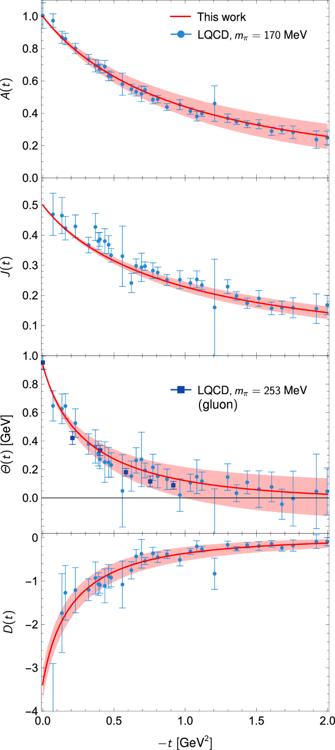
Our predictions are shown as red solid lines. We also show the LQCD results at mπ = 170MeV55 and mπ = 253 MeV56, where the later is purely gluonic. The lattice results of Θ(t) at 170 MeV are obtained from a linear combination of the other three GFFs in ref. 55, with errors added in quadrature.
Fig. 5: Comparison of our result for the nucleon D-term with LQCD predictions55.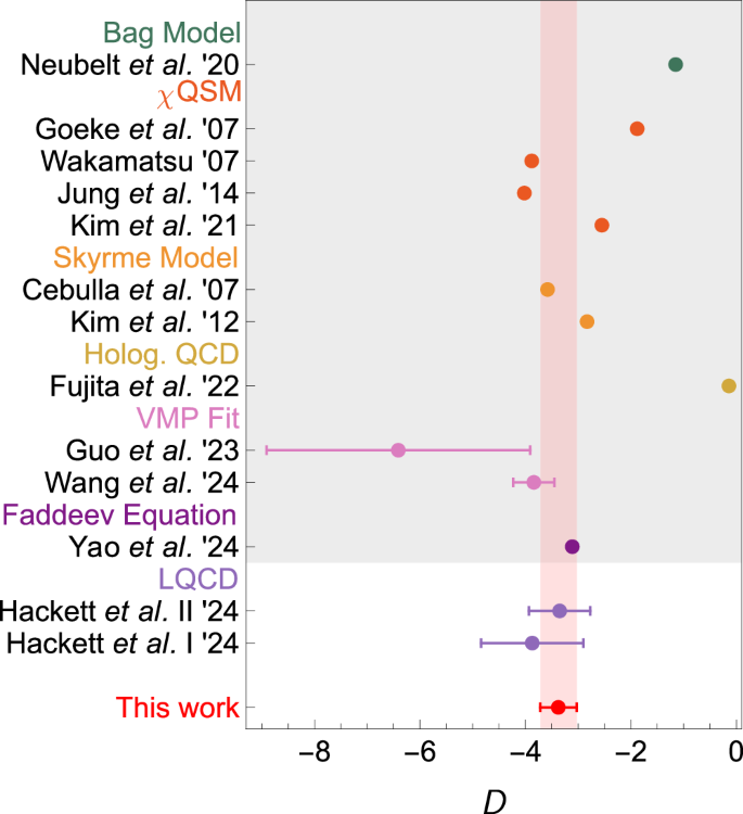
For lattice results, “I” and “II” correspond to extractions therein using tripole and z-expansion fits, respectively. The shaded region includes various model calculations, including Faddeev equation with the rainbow-ladder truncation35, model fits to vector-meson (J/ψ) photoproduction (VMP) data31,32, holographic QCD106, Skyrme model40,42, chiral quark soliton model (χQSM)41,43 —45 and bag model25.
Nucleon radii
Traditional chiral symmetry inspired models describe the proton as a composite system characterized by two scales94: a compact hard core within about 0.5 fm51,95 and a surrounding quark-antiquark cloud (or pion cloud) in which pions play a prominent role. The core carries most of the nucleon mass generated by the (gluonic) trace anomaly, and the pion cloud surrounding this core carries the quantum numbers of the currents, giving rise to the respective form factors. Another influential picture is that a baryon can be viewed as resembling a Y-shaped string, formed by nonperturbative gluon configuration, with valence quarks at the ends96.
Our results strongly suggest that the nucleon should be pictured differently. The mean square radius in the Breit frame of the trace GFF, i.e., derived from the matrix element of \({T}_{\,\mu }^{\mu }\)51, is determined to be
$$\left\langle {r}_{\Theta }^{2}\right\rangle=\frac{6\dot{\Theta }(0)}{{m}_{N}}=6\dot{A}(0)-\frac{9D}{2{m}_{N}^{2}}={\left(0.97\pm 0.03{\mbox{ fm}}\right)}^{2}.$$
(19)
The mass radius, derived from the matrix element of T003, is
$$\left\langle {r}_{{{\rm{Mass}}}}^{2}\right\rangle=6\dot{A}(0)-\frac{3D}{2{m}_{N}^{2}}={\left(0.7{0}_{-0.04}^{+0.03}{\mbox{ fm}}\right)}^{2}.$$
(20)
There are different definitions of the “mass radius” in the literature. In ref. 51, it is given by the radius derived from the scalar trace density, corresponding to rΘ here. However, the term “mass radius” in ref. 97 specifically refers to the quantity derived from the energy or mass density, corresponding to rMass here, while the one derived from the scalar trace density is referred to as the “scalar radius”. We take the latter definition here. A comparison of our results with existing LQCD calculations and model predictions is compiled in Fig. 6. Our results agree with the LQCD results within uncertainties. Given the substantial challenges of direct measurements of GFFs, especially their gluonic components, the dispersive determinations provide invaluable insights into nucleon structure.
Fig. 6: Comparison of our results for the nucleon radius of scalar trace and mass densities with LQCD predictions55,56.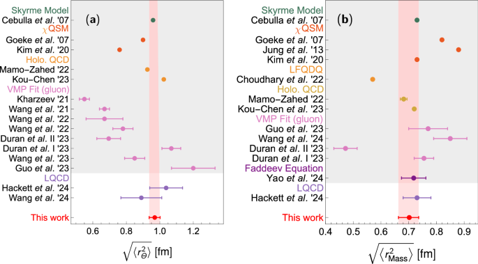
a The shaded region includes results from various models, including model fits to vector-meson photoproduction data31,51,107,108,109,110,111, holographic QCD29,112, χQSM28,41, and Skyrme model40. b The shaded region includes results from various models, including Faddeev equation with the rainbow-ladder truncation35, model fits to vector-meson photoproduction data31,32,107, holographic QCD29,112, light front quark-diquark model (LFQDQ)30, chiral quark soliton model (χQSM)28,41,44, and Skyrme model40. It is noted that the scale dependent results from model fits to vector-meson photoproduction data are purely gluonic.
The nucleon radius of the scalar trace density is sizeably larger than the proton charge radius \(\left\langle {r}_{{{\rm{C}}}}^{2}\right\rangle\), which is \({\left(0.84{0}_{-0.003}^{+0.004}{\mbox{ fm}}\right)}^{2}\) extracted using DRs98 and \({\left(0.84075(64){\mbox{ fm}}\right)}^{2}\) recommended by the Committee on Data of the International Science Council (CODATA)99. The hierarchy in radii suggests, in the sense of Wigner phase-space distribution100,101, that gluons, which are responsible for the majority of the nucleon mass due to the trace anomaly, are distributed over a larger spatial region compared to quarks, which are responsible for the charge distribution. As a quantity characterizing gluonic dynamics in a conventional hadron, the radius of the trace density effectively represents the radius of confinement. In the MIT bag model, this radius may be considered as the bag radius97,102, which serves as a physical boundary of confinement.
It is also instructive to show the nucleon AM39,103 and mechanical radii3,39,100. The former is determined by the combination \(J(t)+\frac{2}{3}t\frac{{{\rm{d}}}}{{{\rm{d}}}t}J(t)\) and the latter by D(t), i.e., \(\left\langle {r}_{J}^{2}\right\rangle=20{J}^{{\prime} }(0)={\left(0.70\pm 0.2{\mbox{ fm}}\right)}^{2},\left\langle {r}_{{{\rm{Mech}}}}^{2}\right\rangle=\frac{6D}{\int_{-\infty }^{0}{{\rm{d}}}t\,D(t)}={\left(0.7{2}_{-0.08}^{+0.09}{\mbox{ fm}}\right)}^{2}\). The results of various radii, together with the error budget, are given in Table 1.
The value of the mechanical radius agrees with recent LQCD results within the uncertainties55,104,105. The observed hierarchy of the radii corresponding to the scalar trace density, the charge distribution, and the AM distribution mirrors the hierarchy in the inverse order of the masses of the lightest mesons excited from the vacuum by the scalar gluon, vector quark-antiquark and tensor currents, respectively, which are σ/f0(500), ρ(770), and f2(1270), respectively. The agreement in the hierarchy ordering suggests a remarkable correlation between the nucleon spatial structure and the light hadron spectrum in the scalar, vector, and tensor channels. It is also stressed in ref. 69 that the LQCD data for the pion GFFs in ref. 75 are fully consistent with the scalar and tensor meson dominance.