Integrated algorithm and hardware design for hybrid neuromorphic systems

Experimental setup

For all experiments, hybrid SNN-ANN models are deployed on two hardware configurations: (1) Jetson-Loihi, where the floating-point ANNs run on Jetson and the SNNs on Loihi, and (2) Edge TPU-Loihi, where an 8-bit quantized ANNs are deployed on the Coral TPU while the SNN runs on Loihi.

Dataset

In our experiments, we use the DvsGesture dataset, which consists of 11 hand gestures recorded from 29 subjects57. DVS events are defined by their type (on/off), pixel location (x, y), and a timestamp. To convert the raw DVS data into a suitable training format, we aggregate all events occurring within a 10 ms window into a 128 × 128 image. Sixteen consecutive images are then stacked to create a single sample with a shape of (2, 128, 128, 16), capturing 160 ms of activity. The dataset includes timestamps indicating when gestures occur, which are used to automatically assign labels to the samples. This preprocessing results in 47,113 training samples and 12,010 testing samples.

AccuracyJetson-Loihi

Figure 1 compares the accuracy of ANN and hybrid SNN-ANN models across three different accumulation intervals: I=2, I=4, and I=8. The results show that ANN models consistently achieve high accuracy with increasing intervals, peaking at 88.36% at I=8. A clear trend emerges among hybrid models, demonstrating their superior performance compared to ANN across all intervals. However, the impact of SpkConv layers varies based on the accumulation interval. At I=8, S1A5 achieves the highest accuracy (88.41%), higher than ANN (88.36%), making it the best-performing model in this setting. At I=2, the hybrid models S2A4, S3A3, and S4A2 achieve close accuracy values of 86.57%, 86.49%, and 86.42% respectively. Among them, S2A4 achieves the highest accuracy, making it the best-performing model at this interval. At I=4, S3A3 achieves the highest accuracy (87.42%), surpassing both ANN and other hybrid models.

Fig. 1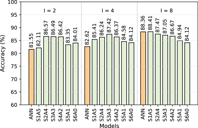

Accuracy analysis for various floating-point ANN, SNN, and hybrid SNN-ANN models on Jetson-Loihi Setup.

These results suggest that at lower accumulation intervals, moderately deep hybrid models with a balanced number of SpkConv layers achieve high accuracy, benefiting from controlled integration of SpkConv layers without significant degradation. However, deeper hybrid models, such as S6A0, experience a slight decline in accuracy, reinforcing the trade-off between accuracy retention and computational efficiency as more SpkConv layers are added.

For SNN-only models, network depth plays a critical role in accuracy. An SNN model with an architecture similar to that of the ANN and hybrid models achieves an accuracy of 55.94%, which is significantly lower than the other two models. However, reducing the network depth mitigates the underfitting issue. For instance, removing one SpkConv layer results in a peak accuracy of 74.24%, though it is still considerably lower than the hybrid model. This emphasizes the importance of hybrid models when aiming for deeper networks, which are often essential for many real-world applications.

Edge TPU-Loihi

We utilize a quantization-aware training strategy to minimize accuracy loss. Each model undergoes 200 epochs of training to achieve optimal performance.

Figure 2 illustrates the accuracy trends of the ANN and hybrid SNN-ANN models across different accumulation intervals I=2, I=4, I=8. The quantized ANN baseline shows a consistent improvement as the accumulation interval increases, achieving 79.16% (I=2), 83.74% (I=4), and 87.83% (I=8). Across all accumulation intervals, hybrid models generally outperform ANN. Notably, S3A3 achieves the highest accuracy of 88.07% at I=2 and 88.05 at I=4, and 88.00% at I=8, highlighting the advantage of a balanced mix of ANN and SpkConv layers. At I=8, the ANN baseline reaches its highest accuracy (87.83%), closely approaching the top-performing hybrid model S3A3 (88.00%). This suggests that while hybrid models maintain an advantage at lower accumulate intervals, at higher intervals, ANN achieves competitive accuracy. This occurs because, at larger accumulate intervals, the temporal information is diminished as more data points in the spike trains are compressed into a single value.

Fig. 2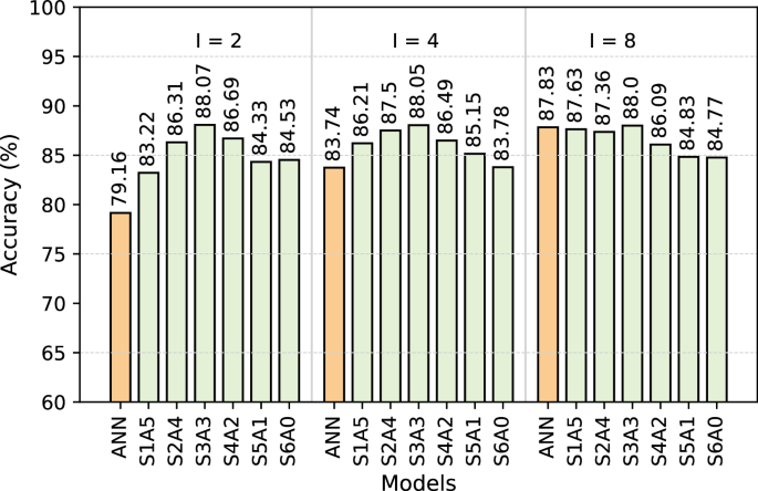

Accuracy analysis for various quantized ANN, SNN, and hybrid SNN-ANN models on Edge TPU-Loihi Setup.

Among hybrid models, S3A3 at I=8, maintains the highest accuracy (88.00%), followed closely by S1A5 and S2A4, demonstrating that hybrid architectures remain effective even at higher accumulation intervals. The performance gap between ANN and hybrid models narrows at I=8, suggesting that models with more ANN layers benefit more from increased accumulation, while hybrid architectures perform better with sparse data (I=2 and I=4). In all cases, beyond the S3A3 configuration, introducing more SpkConv layers cause accuracy reduction, reinforcing the trend that an excessive number of spiking layers introduces inefficiencies that degrade performance. Furthermore, the results indicate that quantized models maintain competitive accuracy, demonstrating that quantization does not significantly degrade model performance, making these models viable for more efficient hardware devices. Furthermore, hybrid models offer an optimal balance between efficiency and accuracy, particularly at moderate accumulation intervals, where they outperform ANN-only models.

LatencyJetson-Loihi

Figure 3 compares the latency of ANN, SNN, and our proposed hybrid SNN-ANN models deployed on Jetson-Loihi setup. Among all the models, the ANN achieves the lowest latency, while the SNN-only model reaches a latency of 32 ms. At I=2, the ANN latency is 1.68 ms, making it 19.04 × faster than SNN. At I=4, ANN achieves a latency of 1.10 ms, leading to a 29.09 × speedup over SNN, while at I=8, it reaches its lowest recorded latency of 0.94 ms, making it 34.04 × faster than the fully spiking model.

Fig. 3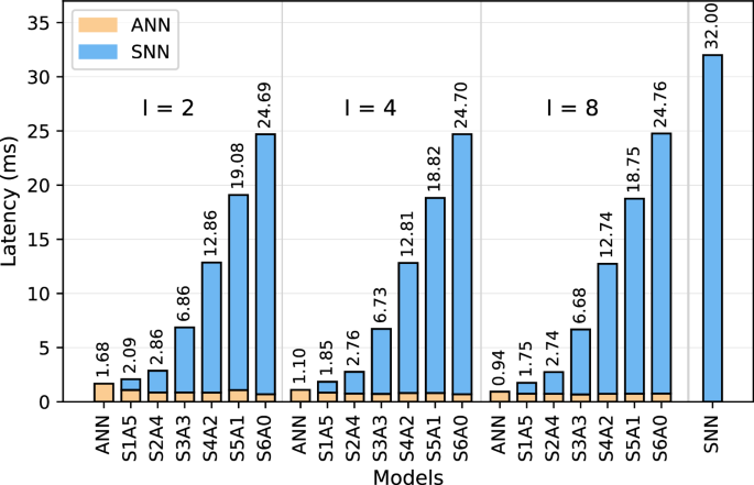

Inference latency for various ANN, SNN, and hybrid SNN-ANN models deployed on Jetson-Loihi setup.

Our hybrid SNN-ANN models leverage the benefits of both ANN and SNN while maintaining a minimal increase in latency. For example, at I=2, S1A5 adds only 0.41 ms compared to the ANN baseline, and at I=8, the delay is only 0.81 ms more than ANN. Increasing I generally reduces latency, except for S6A0, where the latency ranges from 24.69 ms at I=2 to 24.76 ms at I=8. Increasing the number of SpkConv layers generally leads to higher latency. S6A0, the deepest hybrid model, reaches 24.76 ms at I=8, approaching SNN-only latency. However, shallower hybrid models maintain significantly lower latency, making them preferable for optimizing both computational speed and neuromorphic processing efficiency.

Edge TPU-Loihi

Figure 4 presents the latency comparison of different model configurations deployed on Edge TPU-Loihi setup. As shown, increasing the number of spiking layers generally leads to higher latency, with SNN-only models taking the longest latency to process. The quantized ANN baseline demonstrates significantly lower latency, running inference 4.75 × faster at I=2, 8.89 × faster at I=4, and 14.16 × faster at I=8 compared to the SNN baseline. The accumulation interval also plays a crucial role, with ANN latency decreasing from 6.74 ms (I=2) to 3.60 ms (I=4) and further to 2.26 ms (I=8). Hybrid models allow for identifying optimal points where performance is maximized while keeping latency low. Specifically, at I=2, S1A5 achieves 4.28 ms, and with an additional spiking layer, S2A4 further reduces latency to 3.76 ms, making it the best-performing hybrid model in this interval. A similar trend is observed at I=4 and I=8, where S1A5 maintains low latency at 2.92 ms and 2.12 ms, respectively.

Fig. 4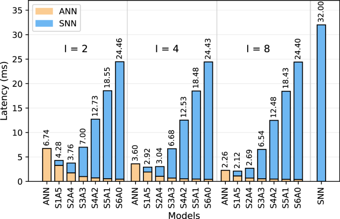

Inference latency for various quantized ANN, SNN, and hybrid SNN-ANN models deployed on Edge TPU-Loihi setup.

The results illustrate that incorporating spiking layers in a controlled manner, as seen in S1A5 and S2A4, provides the best trade-off. These configurations achieve an optimal balance between computational efficiency and the benefits of neuromorphic processing.

Throughput

Table 2 presents the throughput results (in kilo events per second, kE/sec) for ANN, SNN, and hybrid SNN-ANN models across accumulation intervals I=2,4,8, evaluated on both Jetson+Loihi and Edge TPU+Loihi setups.

Table 2 Network throughput

A clear trade-off exists between spiking depth and throughput. As the number of spiking layers increases, throughput decreases. Lightweight hybrids like S1A5 and S2A4 maintain high throughput, while deeper configurations such as S5A1 and S6A0 exhibit significantly lower performance. For example, S6A0 remains nearly constant around 236 kE/sec on Jetson-Nano, regardless of the accumulation interval.

On Jetson-Nano, the ANN model consistently delivers the highest throughput, peaking at 6223.40 kE/s at I=8. In contrast, on the Edge TPU, the performance trend differs: S1A5, a lightweight hybrid model, achieves the highest throughput at both I = 4 and I = 8, reaching 2003.42 and 2759.43 kE/s, respectively. Notably, at I=8, S1A5 outperforms the ANN-only model deployed on the TPU, which reaches 2588.50 kE/s. This indicates that hybrid models with a small number of spiking layers can boost both efficiency and throughput.

At I = 2, S1A5 achieves the highest throughput among hybrid models on Jetson, reaching 2799.04 kE/s, while on the Edge TPU, its performance improves further at higher intervals. This reflects a fundamental difference in how the two platforms respond to accumulation intervals: Jetson benefits from high-speed matrix operations in ANNs and lightweight hybrids even at low I, whereas the TPU gains more from spike aggregation, which reduces memory transfers and enhances efficiency for hybrid models. At I = 4, this contrast becomes more pronounced. Jetson-Nano achieves the highest throughput with the ANN model at 5318.18 kE/s, whereas the Edge TPU performs best with S1A5, which reaches 2003.42 kE/s, outperforming all other models at that interval. This further emphasizes the role of hardware architecture in determining the optimal model configuration for throughput.

Energy consumptionJetson-Nano-Loihi

Figure 5 provides a comparison between the energy across the ANN baselines, SNN baseline, and the hybrid SNN-ANN models across different accumulation intervals. The ANNs consistently exhibits the highest energy usage, peaking at 5.64 mJ at I = 2 and gradually decreasing to 3.22 mJ at I = 8. However, despite this reduction, the ANNs remain the least energy-efficient models, highlighting the need for alternative energy-efficient solutions for edge computing. In contrast, the SNN-only model achieves the lowest energy consumption at 0.64 mJ, highlighting its advantage in energy efficiency. However, this comes at the cost of significantly higher latency 32 ms. These results underscore the trade-offs between computational speed and energy consumption, emphasizing the need for hybrid models to balance both aspects for edge computing.

Fig. 5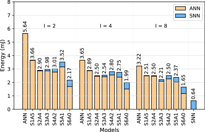

Energy Consumption for various ANN, SNN, and hybrid SNN-ANN models deployed on Jetson-Loihi setup.

Hybrid models consume significantly less energy than ANNs while retaining the computational advantages of ANN components. The results indicate that increasing the number of SpkConv layers generally reduces energy consumption, though this trend is not strictly consistent across all cases. Notably, S6A0 exhibits the lowest energy consumption among hybrid models, decreasing from 2.17 mJ at I = 2 to 1.99 mJ at I = 4, and further to 1.65 mJ at I = 8 achieving a favorable balance between energy efficiency and computational capability. At I = 2, hybrid models’ energy consumption range from 3.66 mJ (S1A5) to 2.17 mJ (S6A0), resulting in up to a 61.5% energy reduction compared to ANN. This trend demonstrates that incorporating SpkConv layers optimally enhances energy efficiency.

Edge TPU-Loihi

Figure 6 compares the energy consumption of the ANNs, hybrid networks, and the SNN-only models deployed on Edge TPU-Loihi setup across different intervals. The results demonstrate that ANN models consume the highest energy in all intervals, e.g., 6.23 mJ at I = 2, while SNN achieves the lowest at just 0.64 mJ. The hybrid models progressively reduce energy usage as more spiking layers are introduced up to a certain point, effectively balancing computational efficiency and energy savings. At I = 2, S6A0 emerges as the optimal hybrid model, consuming 0.88 mJ which is 7.07 × lower than the ANN baseline. Similarly, at I = 4, S5A1 demonstrates the best energy efficiency among hybrid models, consuming just 0.81 mJ, which is 5.06 × lower than ANN. Finally, at I = 8, S3A3 and S5A1 achieve the lowest energy consumption among hybrid models, both at 0.69 mJ, which is 3.65×, lower than ANN. Overall, the results suggest that hybrid SNN-ANN architectures provide a favorable trade-off, enabling significant energy reductions due to the efficiency of SNN layers while retaining performance benefits from the more precise ANN components. These findings highlight the potential of hybrid models for low-power edge AI applications, where balancing computational cost and efficiency is crucial.

Fig. 6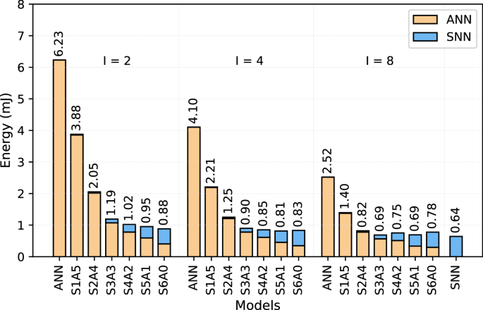

Energy Consumption for various quantized ANN, SNN, and hybrid SNN-ANN models deployed on Edge TPU-Loihi setup.

Accumulator Overheads

By introducing the accumulator between the SNN and ANN models, a small amount of delay and energy overhead is expected due to the added hardware allowing the neuromorphic accelerator to communicate with the ANN accelerator. To measure the latency and energy overhead, an ASIC implementation of the accumulator was designed using the Verilog HDL. This hardware accumulator was then synthesized and tested in Synopsys Design Compiler to attain the overhead of the accumulator at a 100 MHz clock frequency.

The accumulator hardware is implemented by first designing a k-bit counter module along with three control signals: the input clock, reset, and a single-bit input for spikes to be received from the SNN. Here, the parameter k is based on the accumulate interval I. In our experiments, three accumulate intervals of 2, 4, and 8 were tested across the varying hybrid models. Thus, to determine the number of bits to store in each counter the following equation was used:

which results in k = 2, 3, 4 bits, respectively. To allow for all counters in the accumulator to be reset to zero, a single bit was added to the internal register of each counter. In addition to the aforementioned three inputs, the counter also has k output ports to broadcast the accumulated k-bit value to the ANN after I time steps. Thus, for every clock cycle, each k-bit counter accumulates spikes into its internal state register, and after I clocks cycles, the k-bit number is stored for later use by the ANN.

After implementing the single k-bit counter module, a parent accumulator module consisting of N = 128 of these k-bit counters was designed. This accumulator module consists of N = 128 single-bit inputs along with the clock and reset control signals. In our experiments, the input of the accumulator was fixed to N = 128 single-bit inputs, and thus 128 counters, to limit the area of the accumulator to a reasonably realistic size across all hybrid models. The number of output ports for the accumulator module totals 128 × k bits to transfer the accumulated k-bit values of each counter to the ANN accelerator. In addition to the N = 128 counters for accumulating spikes, the accumulator contains a single extra k-bit counter along with a comparator to reset the 128 spike accumulation counters after the I clock cycles have passed.

While N could be set to the total number of neurons in the last layer of the SNN, we found that an accumulator size N = H × W × C in the case of the ANN, N = 128 × 128 × 2, would be rather unrealistic due to the high area and thus energy cost for smaller models with significantly less SNN output neurons. To accommodate models with N > 128, the SNN output neurons are partitioned across the accumulator by dividing the total number of output neurons by N = 128. These partitions are then stored in a memory preceding the accumulator until the accumulator’s controller dispatches the next partition onto the accumulator. Each partition is run for up to T clock cycles. Then a new partition is cycled in, and its accumulated values are saved in a post-accumulator memory for use by the ANN after all partitions have been accumulated.

Table 3 shows the results obtained from Synopsys Design Compiler after synthesizing our accumulator ASIC. The metrics were based on an accumulator input size of N = 128 at a clock frequency of 100 MHz. As listed in the table, the total partitioned accumulator latency ranges from 41 μs, at the most, to 0.64 μs, at the least, throughout the models tested.

Table 3 Accumulator performance results

For energy, Table 3 shows that the accumulator introduces a negligible amount of energy consumption totaling 8.86. nJ in the worst case and 0.0172 nJ in the best case. This shows that while the accumulator does add some latency, energy, and area overheads to the overall system design, it does so only in negligible amounts compared to the total energy consumed during SNN and ANN inference.

Area overheads

Our hybrid SNN-ANN system results have consisted of running experiments on Loihi for the SNN and two edge accelerators, the NVIDIA Jetson Nano and the Google Coral TPU, for the ANN, utilizing a custom accumulator hardware design to integrate the SNN’s output with the ANN’s input. In addition to the areas consumed by the two domains of hardware, SNN and ANN, the accumulator introduces additional hardware overhead into the system. In Table 4, we show the area overheads for each configuration of the accumulate intervals I = 2, 4, 8. The areas of each accumulator interval configuration differ since each accumulate interval is represented by a different number of bits k = log2(I) + 1. Thus, while the input of the accumulator is fixed at 128, the output width differs by a factor of k. In Table 4, the output bit-width of each accumulate interval I = 2, 4, 8 is equal to 256, 384, and 512 bits, respectively, having a direct effect on the total area of the accumulator. As seen in Table 4, as the accumulate interval increases, the area of the accumulator increases.

Table 4 Accumulator area overheadCommunication overheads

Figure 7 shows the communication overhead in terms of latency associated with two different protocols, PCIe and USB 3.0, across various models. It is shown that increasing the number of SpkConv layers reduces communication latency for both the PCIe and USB3 protocols. This reduction occurs because adding more spiking layers halves the size of the feature maps, thereby decreasing the amount of data transmitted by the SNN component to the accumulator with each step. Additionally, using longer intervals further decreases communication latency. For longer intervals, the accumulator aggregates more spikes, thereby reducing the number of bytes sent to the edge device. Consequently, the ANN model with I = 2 exhibits the highest communication latency at 19.76 μs, while the S6A1 model achieves the lowest latency at only 0.21 μs. However, these latency values remain negligible compared to the overall system latency.

Fig. 7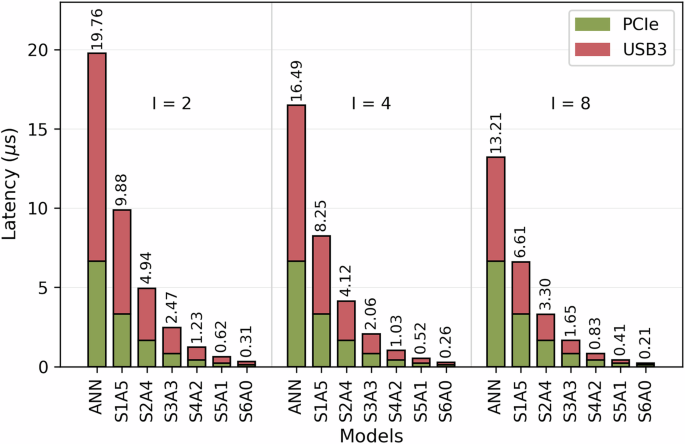

Communication latency overheads.

Figure 8 presents the communication overhead in terms of energy, with the y-axis displayed on a logarithmic scale due to PCIe consuming four orders of magnitude less energy than USB3. The results reveal a clear trend: increasing either the number of SpkConv layers or the interval size significantly reduces communication energy. This is due to the same factors that impact communication latency. Following this pattern, the ANN model with an interval of 2 exhibits the highest communication overhead, consuming 5.29 mJ, whereas the S6A0 model with an interval of 8 achieves the lowest overhead, requiring only 0.04 mJ.

Fig. 8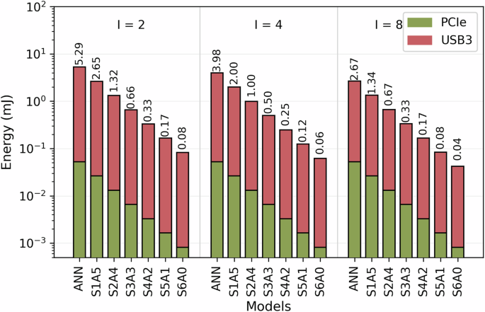

Communication energy overhead.

End-to-end system

Figure 9 shows the percentage contribution of each component to the overall latency of our end-to-end system. The results indicate that the SNN accounts for the majority of the total latency, even in a model like S2A4, which contains only two spiking layers. The accumulator exhibits minimal latency overhead across all evaluated models. In the worst-case scenario—specifically the non-quantized ANN model—the accumulator contributes ~3.6% to the total inference latency. For models ranging from S1A5 to S3A3, this contribution decreases to between 0.1% and 1%. Communication overhead imposes an even smaller latency cost, peaking at ~0.25%. Beyond model S3A3, the combined latency contribution from both the accumulator and communication overhead becomes negligible, consistently falling below 0.001%.

Fig. 9: Latency breakdown of end-to-end system.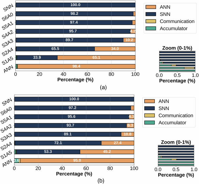

a Latency breakdown for the Jetson-Loihi Setup. b Latency breakdown for the Edge TPU-Loihi Setup.

Figure 10 provides a breakdown of the percentage contribution of each component to the total energy consumption of our end-to-end system. Here, the accumulator is negligible for all models with less than 0.0001% energy. However, the energy consumption of the communication overhead rises dramatically. In all hybrid models with fewer than five spiking layers, the communication overhead exceeds the energy consumption of the SNN. In certain cases, such as S1A5 on the Edge TPU-Loihi setup, the energy overhead is nearly as high as that of the ANN. For the ANN-only model deployed on the Jetson-Loihi setup, the communication overhead even exceeds the processing energy due to the large volume of raw DVS data that must be converted into tensors and transmitted to the Jetson Nano. Additionally, the impact of quantization is more evident, as ANN models mostly consume less energy on the TPU compared to Jetson Nano.

Fig. 10: Energy breakdown of end-to-end system.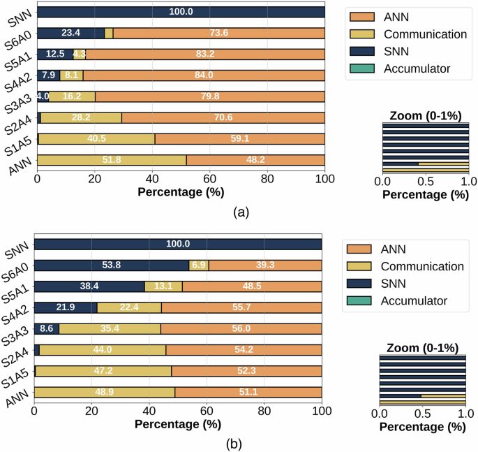

a Energy breakdown for the Jetson-Loihi Setup. b Energy breakdown for the Edge TPU-Loihi Setup.