A description of the experimental development environment and tools is shown in Table 1.
Table 1 Development environment and tools experiment parameter configuration.Dataset and experimental setup
The dataset used in this study is the Tomato Leaf Disease Detection Dataset published on the Roboflow platform. The dataset was split into training, validation, and test sets in a 7:2:1 ratio. All images have a resolution of 640 × 640, with a total of 3,826 images covering seven disease categories: Tomato Early Blight Leaf, Tomato Septoria Leaf Spot, Tomato Leaf Bacterial Spot, Tomato Leaf Late Blight, Tomato Leaf Mosaic Virus, Tomato Leaf Yellow Virus, and Tomato Mold Leaf, along with one healthy class (Tomato Leaf) as a control category.
Considering the relatively limited number of samples in the original dataset, which may restrict the model’s ability to learn effective feature representations, data augmentation was applied only to the training set using three automated techniques provided by the Roboflow platform: horizontal flipping, ± 25% saturation adjustment, and the addition of 0.1% random noise. As a result, the training set was expanded from 2680 to 8040 images, while the validation and test sets remained unaugmented to ensure an objective performance evaluation. The final dataset comprises a total of 9186 images at 640 × 640 resolution. The category distribution of tomato pest and disease samples is summarized in Table 2. These augmentations significantly improved the diversity of training data and enhanced the model’s generalization ability, thereby strengthening its applicability in real-world scenarios. Sample images from the dataset are shown in Fig. 7.
Table 2 Table of category distribution for tomato pest and disease dataset.Fig. 7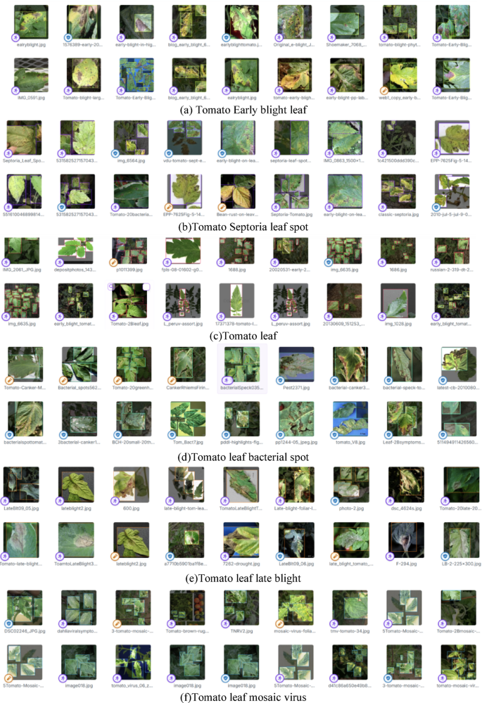
Sample images from the tomato leaf diseases detection dataset.
The batch size was set to 16, and the model was trained for 300 epochs. Stochastic Gradient Descent (SGD) was adopted as the optimizer with an initial learning rate of 0.01 and a momentum parameter of 0.937 to enhance the training performance. The learning rate gradually decayed to 0.001 over the epochs, effectively updating the model parameters and improving performance and accuracy. The detailed parameters are listed in Table 3.
Table 3 Experiment parameter configuration.Performance testing
Figure 8 presents the confusion matrix used to evaluate the performance of various commonly used models, illustrating its object detection accuracy across different categories and providing an intuitive view of the classification accuracy and error analysis. For clarity, the following abbreviations were employed for tomato leaf disease types: Tomato Early Blight Leaf (TEBL), Tomato Septoria Leaf Spot (TSLS), Tomato Leaf (TL), Tomato Leaf Bacterial Spot (TLBS), Tomato Leaf Late Blight (TLLB), Tomato Leaf Mosaic Virus (TLMV), Tomato Leaf Yellow Virus (TLYV), and Tomato Mold Leaf (TML). In addition, BF represents background false positives.
Fig. 8
Confusion matrices corresponding to each evaluated model.
The results shown in Fig. 8 indicate that the DGS-YOLOv7-Tiny model demonstrates excellent performance in detecting various categories of tomato leaf diseases. Compared to the latest YOLOv11s and YOLOv12s models, DGS-YOLOv7-Tiny achieves higher accuracy in detection tasks for most categories. Similarly, when compared to YOLOv8 and YOLOv7, the DGS-YOLOv7-Tiny model also attains superior accuracy across multiple pest and disease categories. Relative to the original YOLOv7-Tiny model, DGS-YOLOv7-Tiny exhibits comparable detection accuracy in most categories, and given the optimization in parameter count and computational complexity, the slight differences in accuracy are negligible. Furthermore, compared with older models such as YOLOv5s and YOLOv3-Tiny, DGS-YOLOv7-Tiny clearly outperforms them in detection accuracy for the majority of pest and disease categories. The detection accuracy for the TLMV category is relatively low across all models, likely due to the similarity of its symptoms to other disease classes and the high overlap of characteristic features. Regarding missed detection rates, most categories perform well; however, the TLYV category exhibits a higher missed detection rate, possibly because the symptoms mainly manifest as mild leaf yellowing and curling, with inconspicuous lesion features, making it difficult for the models to effectively distinguish diseased areas from the background, leading to misclassification. Overall, the DGS-YOLOv7-Tiny model demonstrates strong robustness and generalization capability, delivering outstanding detection performance across the vast majority of disease categories.
In image object detection, the interplay between confidence, F1 score, precision, and recall can be critical for evaluating and optimizing model performance. A comparison of these metrics may help identify areas for improvement. For instance, if the precision is low, the confidence threshold can be raised or false positives minimized. If recall is low, the threshold can be lowered to detect more targets. In practical applications, appropriate metrics and threshold settings should be selected based on specific requirements to achieve optimal detection results.
Precision quantifies the proportion of true-positive instances among all the instances predicted as positive. The calculation formula is shown in Eq. (11).
$${\text{Precision}} = \frac{{{\text{TP}}}}{{{\text{TP}} + {\text{FP}}}}$$
(11)
where TP denotes the true positives, and FP denotes the false positives.
Confidence reflects the model’s certainty regarding the presence of a target in the detection box, with the confidence threshold directly influencing the precision. Raising the confidence threshold typically increases precision but may reduce recall by excluding lower-confidence detections. Conversely, lowering the threshold increases the number of positive predictions, increasing both true positives (TP) and false positives (FP), although FP often increases more rapidly, resulting in reduced precision.
Figure 9 displays the precision-confidence curve of the DGS-YOLOv7-Tiny model. Increasing the confidence threshold reduces false positives, thereby enhancing precision.
Fig. 9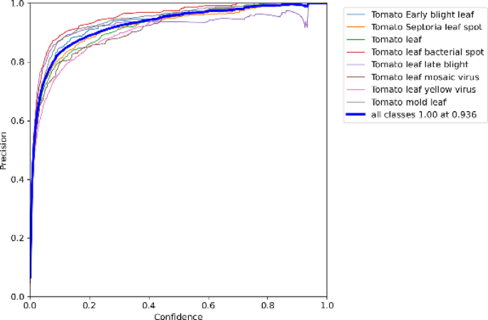
Precision-confidence curve.
Recall quantifies the proportion of true positive instances correctly predicted among all actual positive instances.The calculation formula is shown in Eq. (12).
$${\text{Recall}} = \frac{{{\text{TP}}}}{{{\text{TP}} + {\text{FN}}}}$$
(12)
where FN denotes a false negative.
Unlike precision, the denominator of recall (TP + FN) represents the total number of positive samples, which is fixed. Recall changes only when TP changes. Lowering the confidence threshold classifies more low-confidence samples as positive, increasing TP and recall, but also increasing FP, which reduces precision. Conversely, raising the threshold improves precision but may decrease recall.
Figure 10 shows the recall confidence curve of the DGS-YOLOv7-Tiny model. Lowering the confidence threshold increased the number of detected objects, thereby improving recall. This approach could be beneficial in scenarios requiring high recall to ensure the detection of as many objects as possible.
Fig. 10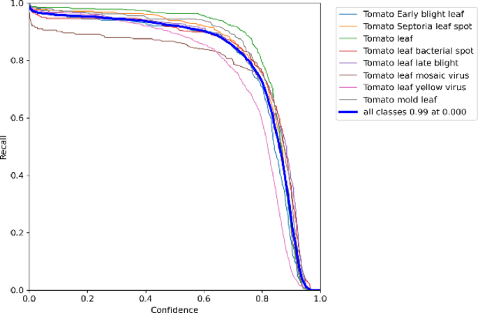
The F1 score, calculated as the harmonic mean of precision and recall, can provide a balanced and comprehensive evaluation of the model’s performance.The calculation formula is shown in Eq. (13).
$${\text{F}}1 = 2 \times \frac{{{\text{Precision}} \times {\text{Recall}}}}{{{\text{Precision}} + {\text{Recall}}}}$$
(13)
Adjusting the confidence threshold can filter the detection results at varying confidence levels, affecting the F1 score. Analyzing the relationship between confidence and F1 score may help determine the optimal threshold to balance precision and recall, maximizing the F1 score. This optimization could be essential for enhancing model performance, improving detection accuracy, and minimizing false positives.
Figure 11 illustrates the F1 score versus confidence curve for the DGS-YOLOv7-Tiny model. In object detection, a higher F1 score reflects better model performance. The confidence threshold filtered the detection results at various confidence levels. A higher threshold reduces the number of detections but increases precision while lowering recall. Conversely, a lower threshold increases the number of detections but may introduce more false positives.
Fig. 11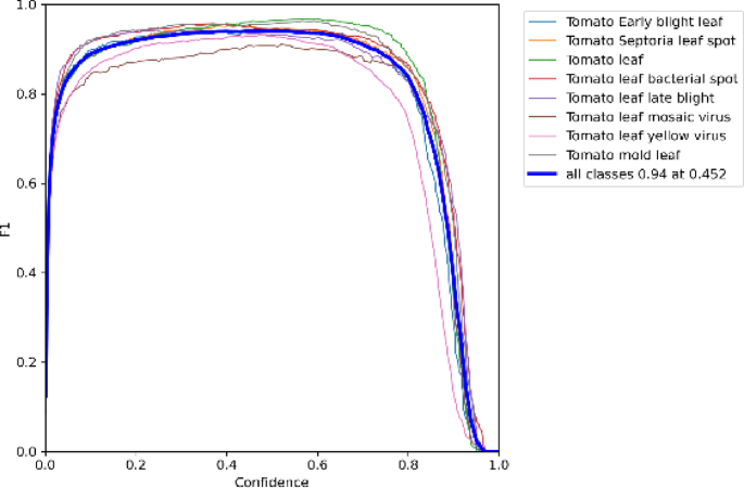
F1 Score-confidence curve.
Figures 9, 10 and 11 illustrate the systematic relationships between confidence, precision, recall, and F1 scores. As confidence increases, precision improves, whereas recall declines. The F1 score peaks when confidence is between 0.4 and 0.6, indicating that the DGS-YOLOv7-Tiny model achieves the optimal balance between precision and recall within this range.
Precision and recall often exhibit a trade-off: increasing recall may decrease precision and vice versa. Adjusting the model parameters or training strategies can improve recall while maintaining precision, or enhance precision while preserving recall. Depending on the application scenario, prioritizing precision may be necessary to ensure result reliability, whereas prioritizing recall may be essential for maximizing target detection.
Figure 12 depicts the precision-recall curve of the DGS-YOLOv7-Tiny model. As recall increased, precision decreased slightly, and the overall performance remained stable. However, when recall approaches 0.9, the precision drops significantly, suggesting that achieving a higher recall may introduce more false positives. Despite this, the DGS-YOLOv7-Tiny model demonstrated excellent performance within a typical range.
Fig. 12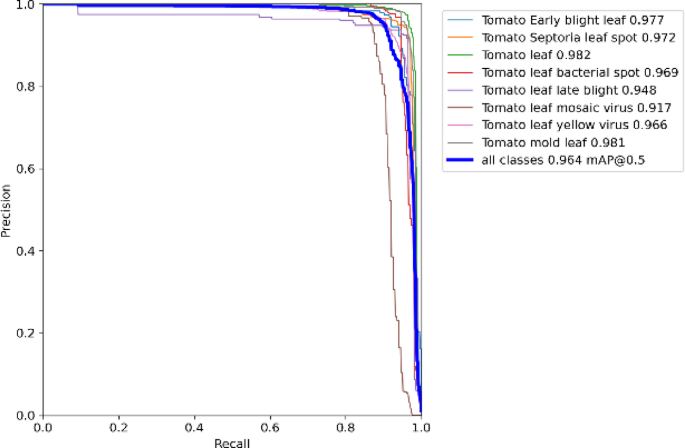
Figure 13 shows the training results for the DGS-YOLOv7-Tiny model. During the first 200 epochs, the loss function value decreased rapidly, whereas precision, recall, and mean average precision (mAP@0.5) increased significantly, indicating a rapid improvement in model performance. Between 200 and 250 epochs, the loss reduction slowed, and the growth of precision, recall, and mAP@0.5 stabilized. Beyond 250 epochs, the training set loss curve exhibited a minimal further decrease, and the other metrics remained stable, suggesting that the model was close to convergence. Although the loss in the validation set was slightly higher than that in the training set, both remained within the same order of magnitude, indicating a strong generalization ability and the absence of significant overfitting.
Fig. 13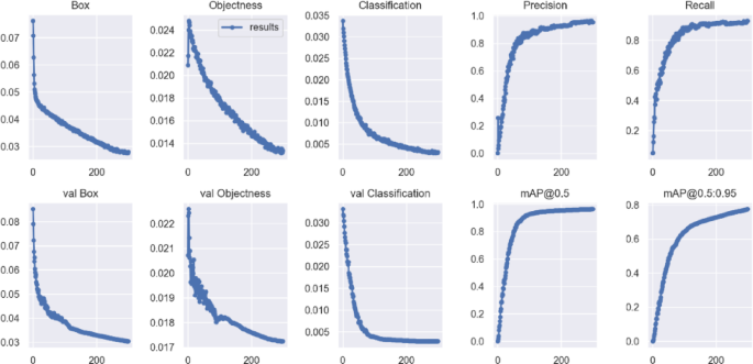
DGS-YOLOv7-tiny training results.
Parameter comparison experiment
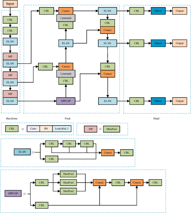
As shown in Table 4, a comparative analysis of the number of parameters between YOLOv7-Tiny and DGS-YOLOv7-Tiny was conducted. In DGS-YOLOv7-Tiny, the module format is denoted as CBS [3, 32, 3, 2], which indicates a convolutional block with the SiLU activation function, an input channel count of 3, an output channel count of 32, a kernel size of 3 × 3, and a stride of 2. In contrast, YOLOv7-Tiny uses CBL [3, 32, 3, 2], where the block adopts the Leaky ReLU activation function, while the other parameters remain the same. In the DGS-ELAN module, the notation “1or3” refers to the use of a 1 × 1 convolution kernel in the CBS block and a 3 × 3 convolution kernel in the corresponding DGSConv block. The term “Global Attention [256]“ denotes a global attention module with 256 input channels.
Table 4 Parameter comparison between YOLOv7-Tiny and DGS-YOLOv7-Tiny.
As shown in the table, DGSConv within the DGS-ELAN module significantly reduces the number of parameters across various output channel configurations. Specifically, when the input and output channels are 256 and 512, respectively, DGS-ELAN reduces the parameter count from 1,838,080 (in the conventional ELAN) to 813,344, achieving a reduction of 1,024,736 parameters, or 55.75%. In the same configuration, the DGSConv module reduces the parameters from 590,336 (in CBL) to 77,968, representing a reduction of 512,368 parameters, or 86.82%. When the input and output channels are 128 and 256, respectively, the parameter count of DGS-ELAN decreases from 460,288 to 205,968, a reduction of 254,320 parameters (55.25%). The corresponding DGSConv module reduces parameters from 147,712 to 20,552, a reduction of 127,160 parameters (86.10%). Similarly, under the configuration of 64 input channels and 128 output channels, the parameters of DGS-ELAN decrease from 115,456 to 52,808, resulting in a reduction of 62,648 parameters (54.26%), while DGSConv reduces the parameter count from 36,992 to 5668, achieving a reduction of 31,324 parameters (84.68%). In summary, DGSConv consistently demonstrates substantial parameter compression across different channel configurations, highlighting its effectiveness in lightweight model design. Moreover, the inclusion of the Global Attention module introduces only a minimal increase in parameters, which is nearly negligible compared to the significant savings achieved by DGSConv.
Ablation experiment
The DGS-YOLOv7-Tiny model demonstrated significant performance improvements across multiple metrics compared with the YOLOv7-Tiny model. A comparison of the evaluation metrics is presented in Table 5.
Table 5 Comparison of key model metrics.
Replacing the Leaky ReLU activation function with SiLU improved the DGS-YOLOv7-Tiny model’s performance compared with the original model, with precision increasing by 1.10% and mAP@0.5 increasing by 0.08%. This improvement was attributed to the SiLU’s enhanced nonlinear expression capability, which increased its stability during training.
Changing the loss function from CIOU to SIOU improved the DGS-YOLOv7-Tiny model’s performance, with precision increasing by 2.72% and mAP@0.5 increasing by 0.19% compared with the original model. This enhancement was primarily owing to the improved object localization accuracy of the SIOU loss function, particularly for targets with uneven scales, where SIOU demonstrated superior performance.
The addition of the Global Attention module improved the DGS-YOLOv7-Tiny model’s performance compared with the original model, with precision increasing by 2.60% and mAP@0.5 rising by 0.56%. This improvement was attributed to the module’s ability to capture global features more effectively, particularly in complex scenarios, thereby enhancing recognition performance.
Replacing the ELAN module with the DGS-ELAN module resulted in a 26.53% reduction in the parameter count and a 1.23% improvement in precision, whereas mAP@0.5 decreased slightly by 0.06%. This modification demonstrated that the model could maintain high detection accuracy while reducing computational costs. In resource-constrained environments, the DGS-ELAN module significantly enhanced efficiency with a minimal impact on performance.
In summary, the slight decrease in mAP@0.5 was outweighed by the improvement in precision and the significant reduction in the parameter count, rendering the change negligible. Therefore, the DGS-YOLOv7-Tiny model demonstrated exceptional performance in agricultural pest and disease detection tasks, achieving a high detection accuracy while maintaining low model complexity.
Comparative experiment
To evaluate the performance of the DGS-YOLOv7-Tiny model for image classification, it was compared with several classic object detection models, including YOLOv3-Tiny, YOLOv5s, YOLOv8s, YOLOv11s, YOLOv12s, YOLOv7, and YOLOv7-Tiny. The experiments plot convergence curves and final detection results using training epochs on the x-axis and mAP@0.5, precision, and recall on the y-axis. The experimental results are shown in Figs. 14, 15, and 16.
Fig. 14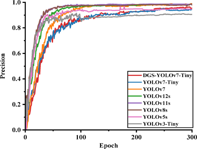
Comparison of precision results for each model.
Fig. 15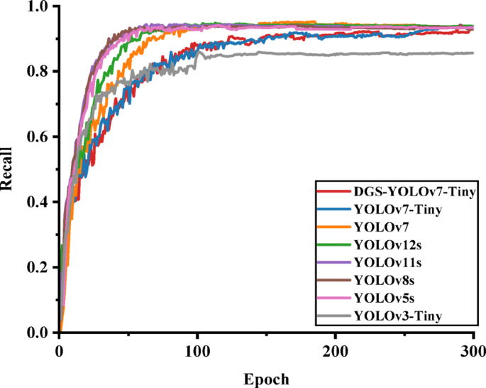
Comparison of recall results for each model.
Fig. 16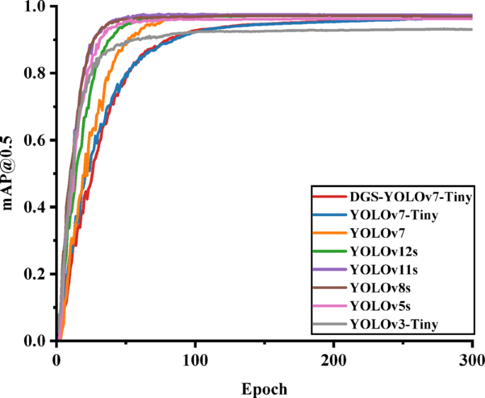
Comparison of mAP results for each model.
Figures 14, 15, and 16 demonstrate that the improved DGS-YOLOv7-Tiny model achieved a comparable or even equivalent performance to the other models in terms of mAP@0.5, precision, and recall. This confirmed that the model sustained high detection performance while delivering greater efficiency.
Table 6 presents a comparison of the evaluation metrics, including precision, recall, mAP@0.5, parameter count, and GFLOPs, for the DGS-YOLOv7-Tiny model and the other models.
Table 6 Comparison of key metrics for different models.
Params and GFLOPs effectively measured the complexity and computational load of the DGS-YOLOv7-Tiny model. As shown in Table 6, the DGS-YOLOv7-Tiny model exceled in both parameter and computational efficiency, with only 4.43 M parameters, 10.2 GFLOPs, and 168 FPS. Compared with YOLOv12s, the model reduces the number of parameters by 51.21%, lowers GFLOPs by 47.15%, and improves inference speed by 64.71%. Compared with YOLOv11s, the parameter count is reduced by 52.97%, GFLOPs decrease by 52.11%, and inference speed increases by 5.00%. Compared with YOLOv8s, the parameter count is reduced by 60.19%, GFLOPs by 64.21%, and inference speed is increased by 15.86%. Compared with the original YOLOv7, the number of parameters is reduced by 88.24%, GFLOPs by 90.74%, and inference speed is improved by 102.41%. Compared with the baseline YOLOv7-Tiny, the model achieves a 26.53% reduction in parameters, a 22.73% decrease in GFLOPs, and a 3.07% improvement in inference speed. Compared with YOLOv5s, the parameters are reduced by 36.99%, GFLOPs by 35.44%, and inference speed is improved by 6.33%. Compared with YOLOv3-Tiny, the model achieves a 48.96% reduction in parameters, a 20.93% reduction in GFLOPs, and a 21.74% increase in inference speed.
Although the DGS-YOLOv7-Tiny model exhibits slightly lower performance in detection accuracy metrics such as Precision, Recall, and mAP@0.5 compared to the more recent YOLOv11s and YOLOv12s models, it achieves approximately 50% reductions in both parameter count and computational complexity, along with a notable improvement in inference speed. Given the emphasis on lightweight design and real-time performance, the slight degradation in Precision, Recall, and mAP@0.5 is considered acceptable.
Presentation of detection results by DGS-YOLOv7-Tiny
To better demonstrate the performance of the proposed DGS-YOLOv7-Tiny model, detection results under the same experimental settings are presented on the validation set of the tomato leaf disease detection dataset, as shown in Fig. 17. Figure 17a, b, c, d, e, f, g and h illustrate the detection results for: Tomato Early Blight Leaf, Tomato Septoria Leaf Spot, Tomato Leaf Bacterial Spot, healthy Tomato Leaf (normal category), Tomato Leaf Late Blight, Tomato Leaf Mosaic Virus, Tomato Leaf Yellow Virus, and Tomato Mold Leaf, respectively. The proposed DGS-YOLOv7-Tiny model exhibits outstanding performance in the field of tomato leaf disease detection, achieving detection accuracy and reliability comparable to human-level diagnosis.
Fig. 17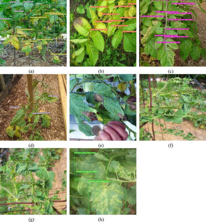
Detection results of tomato leaf diseases.