Chemical reagents
The chemical reagents used in the synthesis experiments include tyrosine (C9H11NO3, 99.0 wt%, Sigma-Aldrich), histidine (C6H9N3O2, 99.0 wt%, Fluka), ciprofloxacin HCl(C17H18FN3O3 ⋅ HCl ⋅ H2O, Merck), n-hexane (C6H14, 97.0 wt%, Honeywell) and distilled water. All chemicals were used without further purification.
Sample preparation and data collection
Single crystals of ciprofloxacin hydrochloride were obtained through vapour diffusion of EtOH/MeCN. These crystals were then directly suspended by sonicating for several minutes. For the sample preparation of amino acids, a small amount of polycrystalline samples was delicately crushed between two microscope slides. The crushed material was then suspended in n-hexane and subjected to ultrasonication for approximately 1 min to achieve uniform dispersion.
Subsequently, a droplet of the resulting suspension was placed onto a TEM grid featuring a lacey carbon film (copper, Ted Pella, 200-mesh). Evaporation of n-hexane was observed with a light microscope. The grid was transferred to an ELSA698 tomography holder (Gatan) at room temperature, which was inserted into the JEM2100Plus TEM (200 keV LaB6, JEOL), equipped with a 1,024 × 1,024 SINGLA 1M detector with an effective area of 1,028 × 1,062 pixels at 75 μm side length per pixel (DECTRIS). The SINGLA detector and the TEM were controlled with the graphical user interface singlaGUI, with source code available on GitHub40. Data were collected at room temperature or 163 K. The beam current was confined with a 50-μm condenser lens aperture and spot size 5. This corresponds to a current of about 20 pA. The sample was illuminated with a beam diameter of about 2.2 μm. Data were collected at 1.0° s−1 and an effective readout rate of 10 Hz (0.1° per frame). The rotation range was up to 140°. In some cases, two or three datasets, with effective detector distances of 860 nm, 1,030 nm and 1,370 mm, were obtained to capture low- and high-resolution data for the samples.
ZSM-5 data were acquired using a JUNGFRAU detector with an effective area of 1,030 × 514 pixels at 75 μm side length per pixel, with the TEM operated by the epoc-GUI graphical interface (source code available on GitHub; ref. 41). Data collection took place at either room temperature or 163 K. A 50-μm condenser lens aperture and spot size 4 were used to confine the beam current. The sample was illuminated with a beam diameter of about 2.2 μm. Data were recorded at a speed of 1.0° s−1, with an effective readout rate of 20 Hz (0.05° per frame). The rotation range extended up to 140°. In some cases, two or three datasets were collected with effective detector distances of 665 mm and 1,025 mm to capture both low- and high-resolution data.
Data processing and model refinement
Data were processed with XDS. The detector distance for each dataset was refined during the CORRECT step of the XDS program to improve the accuracy of the unit cell parameters. The structures were solved by using SHELXT42 for ab initio phasing, followed by refinement and model building using SHELXL and ShelXle, respectively43,44. Full-matrix least-squares refinement with SHELXL using the L.S. command was performed in all cases. Estimated standard uncertainties for all parameters, including the free variables for partial charge assignment, are printed in the SHELXL log file (.lst file) as well as the .mat file, which can be created with the MORE command with a negative parameter. In case of results being combined from multiple datasets, standard uncertainties were estimated as the weighted mean45.
Atomic and ionic electron scattering factors
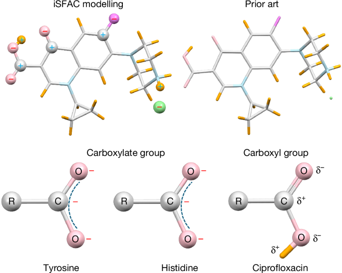
iSFAC modelling of the amino acid structures offered a great revelation underpinning the physical difference between electron and X-ray diffraction. The iSFAC modelling of non-hydrogen atoms includes the electron that the hydrogen contributes to its donor atom. Consequently, as an essential aspect of iSFAC modelling and unlike all other atoms, hydrogen atoms are refined with the scattering factor of H+ (see section ‘iSFAC modelling: quantification of partial charges’ for the technical details). This approach resulted in consistency with chemical intuition and with quantum-mechanical calculations, and at the same time bore some surprises, such as a negative partial charge of the C-atom in carboxylate groups.
Electron scattering factors in Cromer–Mann parametrization,
$$f(s)=c+\mathop{\sum }\limits_{i=1}^{4}{a}_{i}\exp (-{b}_{i}{s}^{2})$$
(1)
suitable for the SFAC command in SHELXL were generated by fitting the Cromer–Mann parameters c, a1, b1, ⋯, a4, b4 against the version of the Mott–Bethe formula published in ref. 22:
$$\begin{array}{l}f(s)\,=\,\frac{{m}_{0}{e}^{2}}{8{\rm{\pi }}{\varepsilon }_{0}{h}^{2}}\frac{{Z}_{0}+\Delta Z-{f}_{{\rm{X}}}(s)}{{s}^{2}}\\ \,\,=\,\frac{1}{8{{\rm{\pi }}}^{2}{a}_{0}}\frac{{Z}_{0}+\Delta Z-{f}_{{\rm{X}}}(s)}{{s}^{2}}\\ \,\,=\,0.02393366{\mathring{\rm A} }^{-1}\frac{{Z}_{0}+\Delta Z-{f}_{{\rm{X}}}(s)}{{s}^{2}}\end{array}$$
(2)
In equation (2), Z0 represents the atomic number of the neutral atom, ΔZ is the additional charge in case of ions, for example, for SiIV: Z0 = 14 and ΔZ = 4, for C−: Z0 = 6 and ΔZ = −1. The term fX(s) is the X-ray scattering factor of the respective atom (not ion), evaluated at the magnitude of the scattering vector s (ref. 46). The terms m0, e, ε and h are the rest mass of the electron, the elementary charge, the dielectric permittivity in vacuum and Planck’s constant, respectively. Equation (2) has the advantage of being suitable for all ions, without dependency on computed X-ray scattering factors for ions such as C− or N+, which may not always be available. Examples of the scattering curves f(s) are shown in Extended Data Fig. 7. Note the offset at high resolution between neutral and ionic scattering curves, which may contribute to the stability of iSFAC modelling. Originally, our first attempts with iSFAC modelling computed fe(s) with the classical Mott–Bethe formula, where the ionic charge is expressed by fX(s) of the ion instead through ΔZ. This, however, did not produce plausible results. Modelling the oxygen of the hydroxyphenyl side chain of tyrosine with either the scattering factor for O− or O+ results in stable refinement, which would mean a negative or a positive partial charge depending on the choice of the crystallographers (data not shown). It was only when scattering factors fe(s) were computed based on equation (2) that iSFAC modelling would unambiguously result in a stable value for the partial charge for all atoms in the model.
In the case of ionic scattering factors, the Cromer–Mann parametrization cannot match the entire resolution range because of the divergence at low resolution (f(s) → ±∞ for s → 0 Å−1). To optimize the fit, the resolution range of the fit was restricted to the resolution range of the particular data sets, 15 Å–0.75 Å in most cases. Note that the Mott–Bethe formula (equation (2)) enables the parametrization of seemingly nonphysical charges, such as O+, C+ or C−, making it suitable for the fitting of positive and negative partial charges for any atom. We used the Levenberg–Marquardt algorithm as implemented in the program GNUPLOT47 for fitting. Future development may result in even better scattering factors, leading to better results from iSFAC modelling48.
iSFAC modelling for quantification of partial charges
We used the program SHELXL for the implementation of iSFAC modelling43. Those who are familiar with the syntax of SHELXL, and thus other programs based on its syntax49, can easily carry out the required steps. Crystallographic refinement compares the observed reflection intensities Iobs(hkl) with calculated intensities Icalc(hkl). In the kinematical approximation, as used by SHELXL, Icalc(hkl) ∝ |Fcalc(hkl)|2. SHELXL is based on the independent atom model, IAM, in which each atom contributes independently to \({F}_{{\rm{calc}}}(hkl)={\sum }_{{\rm{atoms}}j}{f}_{j}(s){{\rm{e}}}^{-8{{\rm{\pi }}}^{2}{U}_{j}(s)}{{\rm{e}}}^{-2{\rm{\pi }}{\rm{i}}{\bf{h}}{{\bf{x}}}_{j}}\), where the sum runs over all atoms in the unit cell. We abbreviated hxj = hxj + kyj + lzj. The subscript j refers to the jth atom, fj(s) is the (element-specific) electron scattering factor of atom j, calculated with the Cromer–Mann parametrization as explained above. The scattering vector s can be computed from the Miller index (hkl). Uj(s) is the isotropic or anisotropic Debye–Waller term, and (xj, yj, zj) are the fractional coordinates of atom j. Conventionally, both the coordinates and ADP values Uj(s) of an H atom are computed from the respective parameters of its geometric environment (AFIX command in SHELXL), rather than refined. iSFAC modelling modifies the conventional handling of H atoms twofold:
-
1.
the partial charge for every non-H atom is computed using a linear superposition between neutral and ionic scattering factor21 and
-
2.
the partial charge for H atoms is computed from their ionic scattering factor.
In the course of our work, we realized that hydrogen atoms have to be included in iSFAC modelling in this special manner. This treatment showed that iSFAC modelling stabilizes H atoms, and their parameters can be freely refined without constraints (possibly supported by mild restraints). When hydrogen atoms are ignored, the resulting partial charges are not very meaningful (Extended Data Fig. 1d, dark red boxes, and section ‘Comparison with quantum-mechanical calculations’). However, when hydrogen atoms are refined as a linear superposition, similar to all other atoms, the refinement does not converge and stops as unstable. Possibly, the scattering factor of H0 is too weak for superposition with the scattering factor of H+. Hence, iSFAC modelling is based on the expression
$$\begin{array}{c}{F}_{{\rm{c}}{\rm{a}}{\rm{l}}{\rm{c}}}(hkl)\,=\,\sum _{{\rm{n}}{\rm{o}}{\rm{n}}\text{-}{\rm{H}}\,{\rm{a}}{\rm{t}}{\rm{o}}{\rm{m}}{\rm{s}}\,j}({\nu }_{j}\,{f}_{j}^{{\rm{i}}{\rm{o}}{\rm{n}}{\rm{i}}{\rm{c}}}(s)+(1-{\nu }_{j}){f}_{j}^{{\rm{n}}{\rm{e}}{\rm{u}}{\rm{t}}{\rm{r}}{\rm{a}}{\rm{l}}}(s)){{\rm{e}}}^{-8{\pi }^{2}{U}_{j}(s)}{{\rm{e}}}^{-2\pi {\rm{i}}{\bf{h}}{{\bf{x}}}_{{\rm{j}}}}\\ \,\,\,\,\,+\,\sum _{{\rm{H}}\,{\rm{a}}{\rm{t}}{\rm{o}}{\rm{m}}{\rm{s}}\,k}{\nu }_{k}\,{f}^{{{\rm{H}}}^{+}}(s){{\rm{e}}}^{-8{\pi }^{2}{U}_{k}(s)}{{\rm{e}}}^{-2\pi {\rm{i}}{\bf{h}}{{\bf{x}}}_{k}}\end{array}$$
(3)
For each atom j, the fraction νj was refined together with its other parameters xj and Uj. Note that each atom was refined individually, and no grouping or other kind of simplification was applied. In SHELXL, the fractions νj and νk are refined through its FVAR mechanism. Equal coordinates and ADPs were imposed with the commands EXYZ and EADP, respectively. This way, iSFAC modelling requires only one extra parameter, νj for each atom in the model.
The fraction νj of the ionic scattering factor for the jth atom in equation (3), and the respective charge offset ΔZ from equation (2) that was used to calculate its ionic scattering factor \({f}_{j}^{{\rm{ionic}}}(s)\) define the partial charge of the jth atom as
$$\delta {q}_{j}={\nu }_{j}\Delta Z$$
(4)
It is noteworthy that refinement with SHELXL can continue only when all free variables fall within the range 0 ≤ νj ≤ 1. In case of negative values, the respective ionic scattering factor can be replaced with its opposite sign, for example, C− with C+ for that particular jth atom. Our study illustrates this feature with the atoms C10, C14 and C18 for ciprofloxacin (Fig. 3). For values >1, the Mott–Bethe formula (equation (2)) allows for the computation of higher oxidation states. Our study shows this feature with the use of scattering factors for SiIV in the case of zeolites.
Cation or anion robustness of assignment
iSFAC modelling does not presume whether an atom is an anion or a cation. We tested both possibilities by replacing the respective ionic scattering factors. If the opposite type was modelled (cation instead of anion, or vice versa), the respective FVAR for the fraction νj would usually go negative. This was the case for the three carbon atoms C10, C14 and C18 in ciprofloxacin. At first, these were modelled with a negative ionic scattering factor similar to all other non-hydrogen atoms. Refinement resulted in negative free variables, which showed the correctness of the opposite sign, that is, a positive partial charge. In some cases, an atom turned out to be neutral, fluctuating about ±0e. This renders the refinement with SHELXL unstable, as SHELXL refuses to start with a negative free variable (although it returns negative occupancy values once refinement has started). In these cases, the partial charge of the atom is set fixed to zero, and its FVAR is unused.
Restraining the total charge using SUMP
Physically, the total charge of the content of a unit cell should be neutral. This knowledge can be added to iSFAC modelling with the SHELXL SUMP command. SUMP is a relatively soft restraint, but in some cases, it reduces parameter shifts. With SUMP, the sum of all partial charges can be restrained to zero. For example, for the amino acid histidine, hydrogen atoms were refined with positive ionic scattering factors and non-hydrogen atoms were refined with negative partial charges modelled with a negative ionic scattering factor. Expressed with the free variable syntax of SHELXL, a neutral molecule satisfies
$$0=-1\times fv({O}_{1})-1\times fv({N}_{1})\ldots +1\times fv({H}_{1})+\ldots +1\times fv({H}_{5})$$
(5)
In SHELXL, this condition can be expressed with the SUMP instruction
SUMP 0 0.001 −1 2 −1 3 −1 4 −1 5 −1 6 −1 7 −1 8 −1 9 −1 10 −1 11 −1 12 1 13 1 14 1 15 1 16 1 17 1 18 1 19 1 20 1 21.
Single crystal X-ray and ED data for Ca tartrate
Tartrate crystals were collected from a glass of Frizzante (2022), vineyard Bioweinbau Thomas Berger, 2212 Großengersdorf, Austria. A crystal was isolated in NVH oil (cat. no. NVHO-1, Jena Bioscience) and mounted on a Bruker D8 diffractometer equipped with a CuKα source (Incoatec) and an EIGER R2 500 detector (DECTRIS). Data were collected with Apex v.3, integrated with XDS and scaled with SADABS50. The structure was solved with SHELXT and refined with SHELXL and the ShelXle GUI. Ionic scattering factors in Cromer–Mann parametrization were produced by fitting the Cromer–Mann function against theoretical X-ray scattering curves, both for the neutral and for ionic forms46,51. ED data from the same batch of crystals were collected at −110 °C, in the same way as the other ED data. Data from 12 crystals were merged to form the final dataset. The samples were very radiation sensitive (possibly because of the presence of four ordered water molecules). Owing to radiation damage, only about 30°–40° of the data were useful from each crystal. The partial charge for Ca2+ was fluctuating around 0.10e, in some cycles close to, but below 0e, which prevents further processing. It was set fixed to 0.10e, similar to the oxygen atom of the water molecule in residue 3 (Extended Data Fig. 6).
Computational approaches to determine partial charges
Numerous methodologies exist for the computation of partial charges in molecular systems. These techniques predominantly rely on electron density1,2,37,52,53,54,55, the electrostatic potential2,38,52,56,57,58 or the electronegativity59 as shown in Extended Data Fig. 1a–c. In the context of electron density-based methods, the partial charge qβ of an atom β is quantitatively defined by the equation
$${q}_{\beta }={Z}_{\beta }-\mathop{\int }\limits_{{V}_{\beta }}\rho ({\bf{r}})\,d{\bf{r}}$$
(6)
Here, Zβ represents the charge of the nucleus, whereas the integral over ρ(R) pertains to the electron density within a specific volume Vβ. Challenges arise in the accurate delineation of this volume, as well as in the distribution of the electron density between bonded atoms. Various methodologies, including those by Mulliken53, Löwdin55, Hirshfeld1,37 (and its successors CM5 and ADCH), Becke60 and NPA54, offer distinct approaches to addressing these issues. The Mulliken population analysis is an archetypal approach, leveraging overlap integrals and the electron density matrix to accomplish this task. Notably, the derived partial charges show a pronounced sensitivity to the choice of basis set. In response, Löwdin population analysis has been developed, using basis set orthogonalization to mitigate basis set dependency, thus enhancing the stability and reproducibility of molecular dipole moments.
The Hirshfeld population analysis represents a marked advancement towards basis set independence. This method deploys a stockholder partitioning mechanism, segregating the electron density predicated on the proportion an atom would contribute within a hypothetical overlay of isolated atomic charge densities. A notable limitation, however, is the dependence of Hirshfeld analysis on atomic reference states. It is worth mentioning that CM5 and ADCH are progressive iterations following the Hirshfeld scheme. Furthermore, NPA operates through natural atomic orbitals derived from a transformation of the molecular wave function. This method offers a more appropriate segmentation, resulting in charge distributions that resonate more intuitively with chemical principles. A caveat to consider with NPA is its elevated computational demand, alongside a potential residual basis set dependency.
Although also based on the electron density, AIM and Becke charges rely on the topology of the electron density rather than molecular orbitals or empirical rules. Becke charges are obtained from a fuzzy atom-centred division of electron density, thereby attenuating the influence of basis set choice. AIM61 divides the molecule into atomic volumes, which allows for a charge determination in equation (6).
By contrast, methods using the electrostatic potential
$$V({\bf{r}})=\sum _{\beta }\frac{{Z}_{\beta }}{| {\bf{r}}-{{\bf{R}}}_{\beta }| }-\int \frac{\rho ({\bf{r}})}{| {\bf{r}}-{{\bf{R}}}_{\beta }| }\,d{\bf{r}}$$
(7)
try to minimize the least-square between V(r) and a charge-based electrostatic potential Vq(r)
$${V}_{q}({\bf{r}})=\sum _{\beta }\frac{{q}_{\beta }}{| {\bf{r}}-{{\bf{R}}}_{\beta }| }$$
(8)
These methods differ in determining points in space to compute the electrostatic potentials. The most popular methods are Merz–Kollman (MK)57, CHELPG56 and RESP38. CHELPG charges often provide values more in line with experimental observations, but the grid quality and placement may notably affect the results62. Alternatively, the RESP methodology incorporates supplementary constraints to enhance the fidelity with which molecular electrostatic attributes are replicated.
Beyond methods that rely on electron density and electrostatic potential, the PEOE model, introduced by Mar and others59, uses electronegativity and ionic potential to distribute partial atomic charges in a molecule.
Quantum-mechanical computations were conducted using Gaussian16 (ref. 28) using the density functionals B3LYP (ref. 63) and ωB97XD (ref. 64). The Pople basis sets 6-31G and 6-311G, along with the Karlsruhe basis set def2-tzvp, were used. We systematically explored all permutations of functionals and basis sets to assess basis set dependence. Geometry optimization started from crystallographic coordinates, and the presence of an energy minimum was confirmed through vibrational frequency analysis. For the amino acids, the zwitterionic state was explicitly enforced. The values for partial charges were derived from Gaussian check files using the MultiWFN 3.8 (ref. 65) software. Notably, except for Mulliken and Löwdin charges, minimal dependence on the selected functional or basis set was observed, aligning with expectations.
Pearson coefficient
The Pearson coefficient is the ratio between the covariance of two datasets (here, the computational and experimental partial charges of atoms within the molecule) and the product of their standard deviations. A Pearson coefficient of one signifies a perfect linear correlation between the datasets.
Generation of electrostatic potential maps
The following steps were taken for the visualization of electrostatic potential maps for tyrosine and histidine, shown in Extended Data Fig. 10.
Experimental ESP maps in CUBE format were exported directly from ShelXle. Experimental maps are scaled to the value F(s = 0), which is ill-defined for ionic scattering factors. Therefore, the value for F(s = 0) from conventional refinement was used by the parameters REM OVERRIDEF000 acknowledged by ShelXle when exporting cube files, for example, the line REM OVERRIDEF000 121.5 was written into the SHELXL instruction file.
The crystallographic RES file was loaded into the program MERCURY (ref. 66). Next neighbours for the central molecule were hand-picked graphically. The resulting composition was exported from MERCURY as an XYZ file. ORCA v.6.0.1 was run in parallel mode from these coordinates with the following script:
where ‘⋯’ was replaced by the content of the XYZ file. ORCA writes a GBW file. This was converted to an input file for MultiWfn with the command
#> orca_2mkl HIS_mrg_4orca -molden
where HIS_mrg_4orca is the basename of the previous ORCA input and output files. This produces the file HIS_mrg_4orca.molden.input, which was used as input to the program MULTIWFN v.3.8 (ref. 65) to compute the ESP and to write this ESP as file totesp.cub in CUBE format. We refer to this CUBE file as totesp.cub, which is the default output name of MULTIWFN. Note that the grid spacing in the QM-ESP and E-ESP cube files is not precisely the same. The Pearson correlation coefficients were computed with the program cubemaps, available on GitHub.
Images in Extended Data Fig. 10 were generated with VMD v.2.0.0a5 as follows. For tyrosine, the colour scaling was set between −0.06 and 0.15 for the E-ESP and between −0.19 and 0.40 for the QM-ESP map. For histidine, the values ranged between −0.04 and 0.09 for the E-ESP and 0.04 and 0.25 for the QM-ESP. The E-ESP maps and the QM-ESP maps were oriented manually to match the following:
First, to load the files, use: File → New Molecule → Browse.
-
1.
Select the electrostatic potential cube file totesp.cub for the QM-ESP.
-
2.
Select the respective cube file exported by ShelXle for the E-ESP, and also load as New Molecule.
Second, for representations, use:
-
1.
Graphics → Representations → Create, Drawing method: CPK
-
2.
Graphics → Representations → Create, Drawing method: Surf; with the following parameters:
For the QM-ESP totesp.cub, it is necessary to select the atoms of the central molecule only. For histidine, these are 20 atoms, INDEX 0 to 19, for tyrosine, these are 24 atoms, INDEX 0 to 23.
Third, for lighting, use:
-
1.
Display → Light 1, Light 2 and Light 3
-
2.
Display → Background → Gradient
Note on simulation software
We computed the ESP and partial charges using the programs ORCA and GAUSSIAN for single molecules, without taking crystallographic symmetry into account. For the ESP comparison of Extended Data Fig. 10, we mimicked crystal space with a next-neighbour approximation. This confirmed the experimental partially charged and the derived ESP. However, for systems that are electronically more complex than the amino acids and metal-organic compounds investigated here, for example, conducting inorganic materials, our approximation might have failed. During peer review, we were made aware of programs that take crystal symmetry into account (for example, NWChem, SIESTA or QUANTUM ESPRESSO) and are more suitable for modelling periodic crystalline systems. We believe future work involving more complex molecules should involve these tools.
Software
The visualization tasks were performed using VMD67, Mercury66 and Platon68.
Computational analyses were conducted using MULTIwfn65,69, ORCA70 with the B3LYP functional and the 6-311G(d) basis set and Gaussian28, following the manuals of these programs.