Universal quantum gate set for Gottesman–Kitaev–Preskill logical qubits

GKP code

Here we give some background on GKP codes, highlighting some of the more salient features in our experiment and simulations. For a more comprehensive summary, see the original proposal6 and more recent reviews48,49. The GKP code is a stabilizer code defined in a bosonic Hilbert space. Its stabilizer generators define a set of lattice points in phase space, which define the code. A family of GKP codes exists, each corresponding to a distinct lattice in phase space46,50. Here we focus on the square GKP code, which is the most fundamental qubit code in this family. The stabilizer generators for this code are given by the two commuting displacement operators

$${\hat{S}}_{X}=\hat{D}(2\alpha ),\quad {\hat{S}}_{Z}=\hat{D}(2\beta ),$$

(2)

where \(\beta ={\rm{i}}\alpha ={\rm{i}}\sqrt{\pi /2}\). These admit the following logical Pauli operators

$${\hat{X}}_{{\rm{L}}}=\hat{D}(\alpha ),\quad {\hat{Y}}_{{\rm{L}}}=\hat{D}(\alpha +\beta ),\quad {\hat{Z}}_{{\rm{L}}}=\hat{D}(\;\beta ),$$

(3)

which commute with the stabilizer generators. Furthermore, a logical CZL gate takes the simple form

$${\hat{{\rm{C}}}}Z_{{\rm{L}}}={{\rm{e}}}^{{\rm{i}}{\hat{q}}_{1}{\hat{q}}_{2}},$$

(4)

where \({\hat{q}}_{j}=({\hat{a}}_{j}+{\hat{a}}_{j}^{\dagger })/\sqrt{2}\) denotes the position operator for mode j.

The code words, which are defined to be the ±1 eigenstates of the stabilizer generators in equation (2), may be expressed in phase space as an infinite sum of coherent states localized at the lattice points defined by α and β:

$$\begin{array}{rcl}\left\vert +{Z}_{{\rm{L}}}^{\;{\rm{ideal}}}\right\rangle &=&\mathop{\sum }\limits_{k,l=-\infty }^{\infty }{{\rm{e}}}^{-{\rm{i}}\pi kl}{\left\vert 2k\alpha +l\beta \right\rangle }_{{\rm{c}}},\\ \left\vert -{Z}_{{\rm{L}}}^{\;{\rm{ideal}}}\right\rangle &=&\mathop{\sum }\limits_{k,l=-\infty }^{\infty }{{\rm{e}}}^{-{\rm{i}}\pi (kl+l/2)}{\left\vert (2k+1)\alpha +l\beta \right\rangle }_{{\rm{c}}},\end{array}$$

(5)

where \({\left\vert \gamma \right\rangle }_{{\rm{c}}}=\hat{D}(\gamma )\left\vert 0\right\rangle\) is a coherent state and |0〉 is the vacuum state. These states are the ±1 eigenstates of ZL, and similar expressions for the ±1 eigenstates of the other logical Pauli operators, \(\left\vert \pm\;{X}_{{\rm{L}}}^{\;{\rm{ideal}}}\right\rangle \,\left\vert \pm\;{Y}_{{\rm{L}}}^{\;{\rm{ideal}}}\right\rangle\), may be obtained by taking superpositions of these states.

Owing to their infinite extent in phase space, these code words have infinite energy. Finite-energy GKP states may be defined by applying the envelope operator onto the infinite energy code words:

$$\left\vert \pm {P}_{{\rm{L}}}\right\rangle =\frac{{{\rm{e}}}^{-{\varDelta }^{2}{a}^{\dagger }\hat{a}}}{{\mathcal{N}}}\left\vert \pm {P}_{{\rm{L}}}^{\;{\rm{ideal}}}\right\rangle ,$$

(6)

where P = X, Y, Z, and \({\mathcal{N}}=\sqrt{\left\langle \pm {P}_{{\rm{L}}}^{{\rm{ideal}}}\right\vert {e}^{-2{\Delta }^{2}{a}^{\dagger }\hat{a}}\left\vert \pm {P}_{{\rm{L}}}^{{\rm{ideal}}}\right\rangle }\). These are approximate ±1 eigenstates of the stabilizer generators and Δ ∈ [0, 1] parameterizes this approximation, with Δ→0 recovering the infinite energy code words. Crucially, the logical operators in equation (3) are not exact logical operators for the finite-energy code words. Methods to construct logical operators that are exact for finite-energy code words via the envelope operator, for example, \({{\rm{e}}}^{-{\varDelta }^{2}{\hat{a}}^{\dagger }\hat{a}}{\hat{Z}}_{{\rm{L}}}{{\rm{e}}}^{{\varDelta }^{2}{\hat{a}}^{\dagger }\hat{a}}\), have been explored for SQ gates in ref. 17 and for the CZL gate in ref. 19.

We stress that the construction for finite-energy GKP states in equation (6) is not unique, and that the exact form of the approximation will depend on the details of the experimental platform that the states are prepared in. This motivates our use of an optimizer to find a logical operation that is tailored to the exact form of the approximate GKP states. However, for numerical purposes, we find an alternative definition for the finite-energy GKP code, which was used in refs. 32,51, particularly useful. Here the code states are defined to be the quasidegenerate ground states of the Hamiltonian

$${\hat{H}}_{{\rm{GKP}}}={\omega }_{0}{\hat{a}}^{\dagger }\hat{a}-J(\cos (2\sqrt{\pi }\hat{q})+\cos (2\sqrt{\pi }\hat{p})),$$

(7)

where \(\hat{q}=(\hat{a}+{\hat{a}}^{\dagger })/\sqrt{2}\) and \(\hat{p}=-{\rm{i}}(\hat{a}-{\hat{a}}^{\dagger })/\sqrt{2}\) are the position and momentum operators for a single bosonic mode, respectively; ω0 represents the characteristic energy scale of the harmonic oscillator; and J quantifies the stabilizer potential enforcing the periodic structure of the GKP code. In the limit of large J/ω0, the ground states are approximately logical Hadamard eigenstates in the |+ZL〉 basis,

$$\left\vert +{H}_{{\rm{L}}}\right\rangle =\cos (\pi /8)\left\vert +{Z}_{{\rm{L}}}\right\rangle +\sin (\pi /8)\left\vert -{Z}_{{\rm{L}}}\right\rangle ,$$

(8a)

$$\left\vert -{H}_{{\rm{L}}}\right\rangle =-\sin (\pi /8)\left\vert +{Z}_{{\rm{L}}}\right\rangle +\cos (\pi /8)\left\vert -{Z}_{{\rm{L}}}\right\rangle ,$$

(8b)

and the squeezing parameter Δ of these states is related to the energy scales through Δ = (ω0/(4πJ))1/4. We find numerical diagonalization of equation (7) to be an efficient procedure to obtain the finite-energy GKP code words numerically. The relations in equation (8) may be inverted to obtain the |+ZL〉 code words, and the other logical Pauli eigenstates obtained from the appropriate superpositions of these states.

Furthermore, the squeezing parameter of these states in each quadrature ΔX/Z may be independently calculated from their stabilizer expectation values through the relations52

$${\Delta }_{X}=\sqrt{-\frac{1}{2\pi }\log \left[| \langle {\hat{S}}_{X}\rangle {| }^{2}\right]},$$

(9a)

$${\Delta }_{Z}=\sqrt{-\frac{1}{2\pi }\log \left[| \langle {\hat{S}}_{Z}\rangle {| }^{2}\right]},$$

(9b)

which can also be expressed in units of decibels, with \({\Delta }_{X/Z}\,({\rm{dB}})=-10{\log }_{10}[{\Delta }_{X/Z}^{2}]\). In this work, we set J/ω0 = 5.95 in equation (7) to target logical states {|+ZL〉, |−ZL〉, |+XL〉, |+YL〉} with squeezing parameters [ΔX, ΔZ] of {[8.39, 7.90], [8.36, 8.88], [7.90, 8.39], [8.38, 8.38]} dB, respectively.

Logical measurements on the GKP code using SSSD

SSSD provides a way to divide the infinite-dimensional Hilbert space into a logical subsystem, containing the logical information encoding in a GKP state, and a gauge subsystem, referred to as the stabilizer subsystem29,53. Here we make use of this formalism to accurately and efficiently readout the logical information encoded in our states.

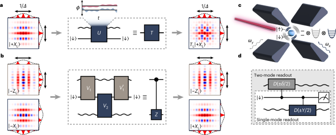
Logical readout for the ideal square GKP code corresponds to measuring the expectation values of the logical Pauli operators, \(\{\langle {\hat{X}}_{{\rm{L}}}\rangle ,\langle {\hat{Y}}_{{\rm{L}}}\rangle ,\langle {\hat{Z}}_{{\rm{L}}}\rangle \}\). The expectation values of these logical Pauli operators are obtained by applying an SDF interaction, which transfers information from the bosonic mode to the ancilla, followed by an ancilla measurement. Setting the phases ϕs and ϕm to be time independent with ϕs = 0, the application of the SDF interaction from equation (1) for a time t realizes the operation \(\hat{D}(\gamma {\hat{\sigma }}_{x}/2)\), where \(\gamma =-{\rm{i}}\Omega t{{\rm{e}}}^{-{\rm{i}}{\phi }_{{\rm{m}}}}\). The magnitude of displacement, |γ|, is controlled by the duration of the SDF pulse, t, and the phase of the displacement, arg(γ), is controlled by the SDF phase, ϕm. Following the SDF pulse, the state measurement of the ancilla gives \(\langle {\hat{\sigma }}_{z}\rangle ={\rm{Re}}[\langle \hat{D}(\gamma (t,{\phi }_{{\rm{m}}}))\rangle ]\), whereas the imaginary part can be obtained by applying an ancilla qubit rotation before the SDF. Setting γ = {α, α + β, β} leads to the measurements of \(\{\langle {\hat{X}}_{{\rm{L}}}\rangle ,\langle {\hat{Y}}_{{\rm{L}}}\rangle ,\langle {\hat{Z}}_{{\rm{L}}}\rangle \}\).

The expectation value of joint Pauli logical operators on two bosonic modes is obtained by applying two sequential SDF operations followed by an ancilla measurement, resulting in \(\mathrm{Re}\,[\langle \hat{D}(\gamma )\otimes \hat{D}(\delta )\rangle ]\).

To decode a GKP state, measuring the Pauli expectation values of finite-energy GKP states with the operators of equation (3) is only valid in the limit Δ→0. As explained in the main text, one can instead measure the expectation value of the Pauli measurement operators, which was done for the SQ gates and Bell state characterization. These operators are defined as a summation over displacement operators on the logical GKP lattice30:

$${\hat{X}}_{{\rm{m}}}=\frac{1}{\pi }\mathop{\sum }\limits_{n=-N}^{N-1}\frac{{(-1)}^{n}}{n+\frac{1}{2}}\hat{D}\left(\alpha \left(2n+1\right)\right),$$

(10a)

$${\hat{Y}}_{{\rm{m}}}=\frac{1}{{\pi }^{2}}\mathop{\sum }\limits_{m,n=-N}^{N-1}\frac{\hat{D}\left(\alpha (2n+1)+\beta (2m+1)\right)}{\left(n+\frac{1}{2}\right)\left(m+\frac{1}{2}\right)},$$

(10b)

$${\hat{Z}}_{{\rm{m}}}=\frac{1}{\pi }\mathop{\sum }\limits_{m=-N}^{N-1}\frac{{(-1)}^{m}}{m+\frac{1}{2}}\,\hat{D}\left(\beta \left(2m+1\right)\right),$$

(10c)

where N sets a truncation, and the identity Pauli measurement operator \({\hat{I}}_{{\rm{m}}}\) coincides with the identity operator on Fock space. The expectation values \(\langle {\hat{X}}_{{\rm{m}}}\rangle\), \(\langle {\hat{Y}}_{{\rm{m}}}\rangle\) and \(\langle {\hat{Z}}_{{\rm{m}}}\rangle\) are obtained by summing over the expectation values of the displacement operator, \(\langle \hat{D}(\gamma )\rangle\). Here γ is varied to sample the various points determined by equation (10). Expectations of joint Pauli measurement operators for two bosonic modes, such as \(\langle {\hat{X}}_{{\rm{m}}}\otimes {\hat{Z}}_{{\rm{m}}}\rangle\), can be obtained by taking the tensor product of any two single-mode Pauli measurement operator of equation (10). Their joint expectation value will also be a summation over the expectation values of two-mode displacement operators.

The number of required measurements is reduced by using the fact that \(\langle \hat{D}(\gamma )\rangle ={\langle \hat{D}(-\gamma )\rangle }^{* }\). With this, the total number of measurements to calculate the three single-mode expectation values of the Pauli measurement operators of equation (10) is Nmeas = 2N + 2N2. For the expectation values of the 15 non-trivial two-mode Pauli measurement operators, the number of measurements is Nmeas = 4N + 8N2 + 8N3 + 4N4. The finite-energy envelope of the GKP states implies that \(\langle \hat{D}(\gamma )\rangle \approx 0\) for large enough |γ|, meaning that the sums in equation (10) converge with N. In both SQ gate and Bell state experiments, we choose a truncation of N = 2 to minimize the number of measurements required, but still achieve a good approximation (in Supplementary Section C, we quantify the error arising from this truncation). This results in Nmeas = 12 and Nmeas = 168 measurements for logical SQ and TQ states, respectively. For the CZL gate experiment, we choose not to measure the Pauli measurement operators because the required number of measurements for all 16 states is 2,688, leading to a much longer experimental runtime. Instead, we choose to measure the expectation values of the logical Pauli operators of equation (3), which requires a total of 240 measurements, and incorporate the error from using these operators into our error budget (Supplementary Fig. 3).

State tomography

In the SQ experiment, the logical density matrices \({\hat{\rho }}_{{\rm{L}}}^{{\rm{in}}}\) and \({\hat{\rho }}_{{\rm{L}}}^{{\rm{out}}}\) are reconstructed from the Pauli measurement expectation values using the relation

$${\hat{\rho }}_{{\rm{L}}}=\frac{1}{2}{\hat{E}}^{0}+\frac{1}{2}\mathop{\sum }\limits_{i=1}^{3}\left\langle {\hat{E}}_{{\rm{m}}}^{i}\right\rangle {\hat{E}}^{i},$$

(11)

where \({\hat{E}}^{i}\in \{\hat{I},{\hat{\sigma }}_{x},{\hat{\sigma }}_{y},{\hat{\sigma }}_{z}\}\) are the usual one-qubit Pauli operators and \({\hat{E}}_{{\rm{m}}}^{i}\in \{{\hat{I}}_{{\rm{m}}},{\hat{X}}_{{\rm{m}}},{\hat{Y}}_{{\rm{m}}},{\hat{Z}}_{{\rm{m}}}\}\) are the Pauli measurement operators, which can be obtained from the experiment using equation (10). We construct a tomographically complete set of \({\hat{\rho }}_{{\rm{L}}}^{{\rm{in}}}\) by preparing one of the four states {|+ZL〉, |−ZL〉, |+XL〉, |+YL〉} and taking measurements for each of the expectation values in equation (11), leading to a total of 4 × 12 = 48 measurements (Supplementary Section B). Reconstructing each \({\hat{\rho }}_{{\rm{L}}}^{{\rm{out}}}\) is performed in a similar manner, but with the gate applied to each initial state.

In the TQ experiment, the input and output density matrices are reconstructed from Pauli expectation values using the relation

$${\hat{\rho }}_{{\rm{L}}}=\frac{1}{4}{\hat{E}}^{0}+\frac{1}{4}\mathop{\sum }\limits_{i=1}^{15}\langle {\hat{E}}_{{\rm{L}}}^{i}\rangle {\hat{E}}^{i},$$

(12)

where \({\hat{E}}^{i}\in {\{\hat{I},{\hat{\sigma }}_{x},{\hat{\sigma }}_{y},{\hat{\sigma }}_{z}\}}^{\otimes 2}\) are the TQ Pauli operators and \({\hat{E}}_{{\rm{L}}}^{i}\in {\{{\hat{I}}_{{\rm{L}}},{\hat{X}}_{{\rm{L}}},{\hat{Y}}_{{\rm{L}}},{\hat{Z}}_{{\rm{L}}}\}}^{\otimes 2}\) are the logical Pauli operators of equation (3). We first reconstruct each \({\hat{\rho }}_{{\rm{L}}}^{{\rm{in}}}\) by preparing one of the 16 possible input states from the set {|+ZL〉, |−ZL〉, |+XL〉, |+YL〉}⊗2 and measuring the 15 different non-trivial logical Pauli operators, resulting in 16 × 15 = 240 measurements. Similarly, each \({\hat{\rho }}_{{\rm{L}}}^{{\rm{out}}}\) is retrieved by applying the CZL gate after preparing one of the input states.

The Bell state is characterized using logical QST, which aims to reconstruct the logical density matrix of the experimentally prepared state. In the Bell state experiment, we reconstruct the logical density matrix from

$${\hat{\rho }}_{{\rm{L}}}=\frac{1}{4}{\hat{E}}^{0}+\frac{1}{4}\mathop{\sum }\limits_{i=1}^{15}\langle {\hat{E}}_{{\rm{m}}}^{i}\rangle {\hat{E}}^{i},$$

(13)

where \({\hat{E}}^{i}\in {\{\hat{I},{\hat{\sigma }}_{x},{\hat{\sigma }}_{y},{\hat{\sigma }}_{z}\}}^{\otimes 2}\) are the TQ Pauli operators and \({\hat{E}}_{{\rm{m}}}^{i}\in {\{{\hat{I}}_{{\rm{m}}},{\hat{X}}_{{\rm{m}}},{\hat{Y}}_{{\rm{m}}},{\hat{Z}}_{{\rm{m}}}\}}^{\otimes 2}\) are the Pauli measurement operators. The expectation values are calculated from equation (10), where a truncation of N = 2 results in 168 unique measurements. We apply a post-processing step in the logical Bell state analysis, ensuring that the reconstructed state is physical. After obtaining \({\hat{\rho }}_{{\rm{L}}}\) from equation (13), we use a convex optimizer to obtain a physical density matrix, \({\hat{\rho }}_{{\rm{L}},{\rm{Bell}}}\), which minimizes \(| | {\hat{\rho }}_{{\rm{L}},{\rm{Bell}}}-{\hat{\rho }}_{{\rm{L}}}| {| }_{2}\) (ref. 54). \({\hat{\rho }}_{{\rm{L}},{\rm{Bell}}}\) is constrained to be non-negative definite and \(\mathrm{Tr}\,({\hat{\rho }}_{{\rm{L}},{\rm{Bell}}})=1\). Expectation values of the physical density matrix \({\hat{\rho }}_{{\rm{L}},{\rm{Bell}}}\) are plotted in Fig. 4.

Uncertainty analysis

Uncertainties on the logical fidelities presented in this work are determined using a non-parametric bootstrap procedure. For each dataset, we resample the raw spin readout counts with replacement to create 1,000 pseudo-datasets of identical size. Each resampled dataset is processed through the full analysis: first extracting the relevant displacement operator expectation values, then reconstructing the logical density matrix or process matrix and finally calculating the fidelity metric. The standard deviation of the resulting distribution of 1,000 fidelity values is taken as the one standard deviation (1σ) statistical uncertainty reported in the main text.

Calibration and experimental drift

To mitigate errors from slow experimental drifts, we implement an interleaved calibration routine throughout the experiment. The motional mode frequencies ωx and ωy, corresponding to the radial-x and radial-y modes, are periodically recalibrated approximately every 30 s using a calibration protocol described in ref. 55. Independent measurements reveal that the frequency drifts by σδ ≈ 2π × 3.2 Hz between calibrations, and that drifts in ωx and ωy are highly correlated. We estimate errors due to frequency drifts from numerical simulations by repeating a similar analysis, as carried out in Supplementary Section C. The SDF Hamiltonian in equation (1) is modified by adding a noisy Hamiltonian term of the form \({\delta }_{x}{\hat{a}}_{1}^{\dagger }{\hat{a}}_{1}+{\delta }_{y}{\hat{a}}_{2}^{\dagger }{\hat{a}}_{2}\). We set δ = δx = δy to model-correlated frequency drifts, and \(\delta \approx {\mathcal{N}}(0,{\sigma }_{\delta }^{2})\) is sampled from a normal distribution. The resulting infidelity is below 5 × 10−3 across all experiments.

By contrast, drifts in the qubit frequency and SDF Rabi rate occur on much slower timescales and are not included in the scheduled calibration routine. These parameters do not appreciably drift over the duration of the experiments and have a negligible impact on the fidelities relative to drifts in the motional frequency.