This section explains the proposed CRFTS model, which uses a clustering approach for allocation and the advance reservation of VMs to handle the failure in a dynamic, computationally intensive cloud system. The proposed cluster-based allocation technique can be represented as a bipartite graph between the task set and VM set, as shown in Fig. 1. Additionally, the notions used are presented in Table 3. The System Model and Problem Formulation are illustrated in the subsection below. In this section, we introduced the fault-tolerant-based scheduling algorithm. The incoming tasks are represented as set T= {t1, t2, t3… tn} and the VMs are represented as set V= {v1, v2, v3… vk}. At any decision point (t), only subset Tk of T, i.e., Tk ⊆ T, is known. Since the entire task set T is unknown, the scheduler must make decisions without prior knowledge of tasks, which models the problem as online scheduling. The proposed scheduling assigns each arriving task to a VM based only on the current system state.
Fig. 1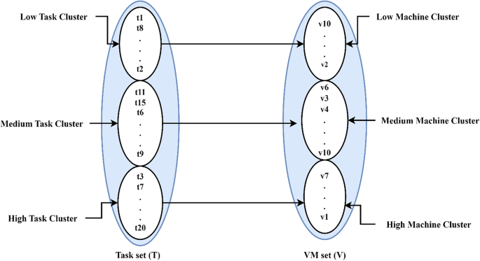
Clustered-allocation mapping strategy.
System model
The CRFTS system architecture includes several components, as illustrated in Fig. 2. User tasks are submitted to the Application Layer. Besides, in the cloud, the tasks may come from any geographical location at any point in time. The Task Sorter sorts the incoming tasks in ascending order of task size. Similarly, the Host/VM Layer contains a variety of resources with varying processing abilities. VM Sorter sorts the available VMs in ascending order of their processing abilities. Additionally, the sorting of both tasks and VMs is followed by a clustering mechanism where both tasks and VMs are separated into three different clusters, i.e., low, mid, and high clusters, as discussed in the algorithm section. The clustering will further ensure the best-suited task and VM mapping by limiting the task and VM domain of mapping. Furthermore, the VM allocator is responsible for choosing the relevant VM from the cluster for task completion.
Each VM periodically sends a simulated heartbeat signal at a fixed interval δ. The heartbeat controller records the last received time Hj of the signal. If the difference between current time τ and Hj exceeds a threshold “Δ”, the VM is considered faulty and the tasks on it are marked as failed and rescheduled accordingly.
The AR Module/Fault Handler collaborates with the VM Allocator and the Heartbeat Monitor to detect and manage VM and task failures, initiating reservations to ensure the uninterrupted execution of tasks. This coordination guarantees fault-tolerant execution with minimal downtime. The VM allocator also communicates the generated schedule to the AR Module. In response, the AR Module’s Time Manager component predicts the AR slot as given in Eq. 3 based on the schedule produced by the VM allocator. The Reservation Producer component provides the alternative VM for the computed AR slot in case of a fault, thereby initiating the reservation.
Fig. 2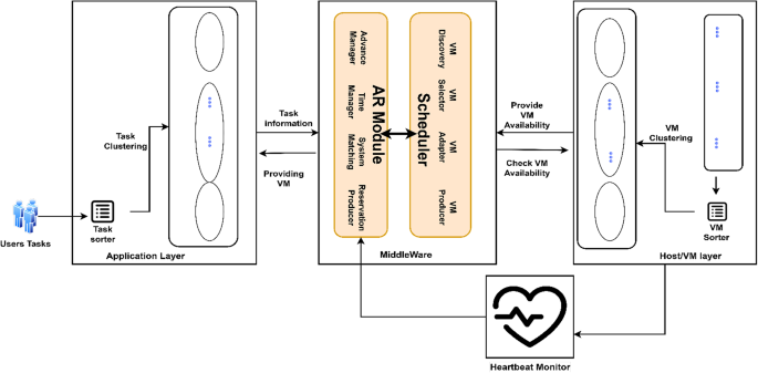
System architecture of CRFTS.
Problem formulation
The section presents a foundation for the rest of the work, facilitating readers to understand the objectives, variables, constraints/assumptions, and approach of the research done in the work.
Task and VM Constraints/Assumptions:
\(1MI~ \leqslant ~Size{\text{ }}({t_i}) \leqslant 100MI\)
\(1MIPS~ \leqslant ~Speed{\text{ }}({v_j}) \leqslant 100MIPS\)
Objectives of the model: Minimize makespan while maximizing resource utilization and reliability.
Allocation Variables: STij, FTij, Rj, P(ti,vj).
Fault Tolerance Variables: AR, ARM, Status.
The allocation and fault tolerance variables are calculated in the problem formulation section later. The task allocation problem is modelled mathematically as a mapping of every arriving task to the suitable VM cluster to optimize reliability. The proposed model works in five phases:
Phase 1: task clustering
This phase is responsible for organizing the tasks in three clusters, namely, Low task Cluster, Medium task Cluster, and High task Cluster.
Phase 2: VM clustering
This phase is responsible for organizing the VMs in three clusters, namely, Low VM Cluster, Medium VM Cluster, and High VM Cluster.
Phase 3: task to Vm mapping without reservation
In each cluster, the VMs and tasks may be placed in random order because the task and VM clusters are created based on task size and VM speed, respectively, and not based on the number. Mathematically, the mapping (µ) can be represented as follows:
µ: T → V
Every task has its Start time and Finish time, which are computed in Eqs. (1) and (2). To reserve the VM, the task execution time slot, i.e., the AR slot for every task on a suitable VM, is estimated. The AR slot for each task is calculated by taking the difference between ST and FT as computed in Eq. (3). The ST is the time when the task starts executing on the allocated VM. The FT is the time when the task completes its execution on that VM. The execution time of the task is added to the ST of that task to compute the FT. Additionally, each VM has a load history (Rj) that is used to determine when it is ready to execute the new task. Whenever any ti will begin to execute on any vj after mapping according to the allocation procedure. The time at which the allocation of ti begins or starts on vj is known as STij. Rj is first assumed to be STij as seen in Eq. (1)
$$S{T_{ij}}={\text{ }}{R_j}$$
(1)
Once ti has completed its execution on vj, the processing time of ti on vj (p(ti, vj)) is added to the STij as indicated in Eq. (2) to determine the FTij.
$$F{T_{ij}}={\text{ }}S{T_{ij}}+{\text{ }}p\left( {{t_i},{v_j}} \right)$$
(2)
$$AR\,=\,F{T_{ij}} – {\text{ }}S{T_{ij}}$$
(3)
Here, p(ti,vj) is computed by dividing the size of ti by the speed of vj.
Phase 4: failure modelling and detection via heartbeat mechanism
The model enables every VM to send a heartbeat signal at certain instances (Hj).
Parameters defined for enabling the heartbeat mechanism:
δ: Heartbeat interval (VM sends the heartbeat every δ units of time), Hj: Last heartbeat timestamp from VM.
T: Current time, Δ: Timeout threshold.
The heartbeat mechanism works in two steps:
Step 1: Heartbeat Sending
The phase initially tracks the time of sending the heartbeat by using the δ as:
\(T{\text{ }}\bmod {\text{ }}\,\delta =\,0\)
If the heartbeat sending time is detected, then VM sends the heartbeat time stamp to the heartbeat controller. After receiving a heartbeat, the controller updates Hj of the corresponding VM with the current time (τ).
\(H\left( {{v_j}} \right){\text{ }}=\tau\)
Step 2: Heartbeat Scanning
The heartbeat controller performs this phase, and it periodically scans the heartbeat of VMs. If the heartbeat of any VM is not found within the time, then it is declared as faulty and ejected from the cluster. The controller measures the past time since the most recent heartbeat was acknowledged from the VM and uses this interval as a pointer for detecting VM failure as:
\(Last\_Breath\,=\,\tau –H\left( {{v_j}} \right)\)
If the Last_Breath exceeds the timeout threshold, then the controller declares the VM as failed by indicating the following:
\(H\left( {VM} \right) = \left\{ \begin{gathered} 1,~~\,\,if~heartbeat~received~from\,~VM~within~Timeout \hfill \\ 0,\;\;\;\;\;\;\;\;\;\;\;\;\;\;\;\;\;\;\;\;\;\;\;\;\;\;\;\;\;\;\;\;\;\;\;\;\;\;\;\;\;\;\;\;\;\;\;\;\;\;\,\,\,Otherwise \hfill \\ \end{gathered} \right.\)
Phase 5: fault tolerance via reservation
In this phase, Task VM mapping is performed, and simultaneously, VMs are monitored for faults using the heartbeat mechanism. In case of faults, advance reservation is enabled and an alternative VM is provided to the affected task. If any VM leaves the system or fails at any point in time, and fault tolerance is not there, the associated tasks may suffer premature termination. The problem is addressed by accompanying the scheduling with a proactive, advance reservation fault tolerance technique. Let’s suppose ‘f’ VMs are failing and these ‘f’ VMs are taken as a separate set of failed VMs (Vf) and are defined as:
\({V_f}={\text{ }}\{ {v_f}:{\text{ }}{v_f} \in V{\text{ }}and{\text{ }}\left| {{V_f}} \right|{\text{ }}=f\}\)
This failure of VMs will affect the corresponding tasks and cause them to fail. Let ‘u’ be the number of unsuccessful tasks. Similarly, these ‘u’ unsuccessful tasks are taken as a separate set of unsuccessful tasks (Tu) and are defined as:
\({T_u}={\text{ }}\{ {t_u}:{\text{ }}{t_u} \in T{\text{ }}and{\text{ }}\left| {{T_u}} \right|{\text{ }}={\text{ }}u{\text{ }}\& {\text{ }}u
Now, these unexecuted tasks need to be reassigned to some alternative VM to complete their execution, which is done by the advance reservation technique. All tasks in Tu are migrated to another VM (Vj) having the least RT from (Vf) for the calculated AR slot such that Vj ∉ Vf as discussed in Algorithm 5.
The proposed clustering approach allocates tasks in three ways. First, sorting helps the model to achieve a one-to-one suitable order. Thereafter, clustering before allocation restricts the domain of allocation, which allows the model to assign the most appropriate VM to the task. Lastly, the task from each cluster is allocated to the corresponding VM clusters only, which helps the model to avoid under- and overutilization of the VM up to a certain degree. However, there are still chances of over- and underutilization of VMs, which will be handled by integrating the proposed approach with an efficient load-balancing technique that is under consideration for future work, which continuously monitors the under- and over-utilizing VMs and shifts the load between them.
Performance metrics
After the successful task execution, the reliability of the system is checked. Additionally, the makespan is taken as the highest or maximum among all TETj and can be expressed as Eq. (4)32.
$$Makespan\,=\,\hbox{max} {\text{ }}\left( {F{T_{ij}}} \right),\forall {V_j}$$
(4)
Progress percentage of makespan (Ppm): It is the percentage of progress in makespan offered in proposed CRFTS over the other existing approaches, i.e., HEFT, E-HEFT, and LB-HEFT approaches, and is calculated in the Eq. (5)33.
$$P{p_m}\left( \% \right){\text{ }}=\frac{{M~\left( {Compared~Approach} \right) – ~M\left( {\Pr oposed~Approach} \right)}}{{M\left( {Compared~Approach} \right)}}*{\text{ }}100$$
(5)
Average of (Ppm): To calculate the deviation from the desired rate in percentage, divide the sum of every Ppi for each tested VM by their respective tested numbers, as shown in the Eq. (6)34.
$$Average{\text{ }}of{\text{ }}\left( {P{p_m}} \right){\text{ }}=\frac{{\mathop {{\text{ }}\sum }\nolimits_{{i=1}}^{t} Ppm~\left( {each~tested~VM~EquationNumber} \right)}}{t}$$
(6)
The Average VM utilization of the system is calculated in the Eq. (7) as35.
$$UT=\frac{{\mathop \sum \nolimits_{1}^{k} \left( {FT~ – ~p\left( {tf~\hbox{c}{\kern-6.5pt}\raise2.75pt\hbox{\vrule height .5pt width3.5pt depth0pt}{\kern4pt}~Tf~,~Vj~\hbox{c}{\kern-6.5pt}\raise2.75pt\hbox{\vrule height .5pt width3.5pt depth0pt}{\kern4pt}~Vf~} \right)} \right)}}{{k~*Makespan}}~\forall Vj~$$
(7)
Progress percentage of UT (Ppu): It is the ratio defining the progress percentage of average utilization of the proposed CRFTS and other compared approaches and is calculated in the Eq. (8) as36.
$$P{p_u}\left( \% \right){\text{ }}=\left( {\frac{{UT~\left( {Compared~Approach} \right) – ~UT\left( {\Pr oposed~Approach} \right)}}{{UT\left( {Compared~Approach} \right)}}} \right)*{\text{ }}100$$
(8)
Average of (Ppm): To calculate the deviation from the desired rate in percentage, divide the sum of every Ppu for each tested VM by the respective number of tests, as shown in the Eq. (9)37.
$$Average{\text{ }}of{\text{ }}\left( {P{p_u}} \right){\text{ }}=\frac{{\mathop \sum \nolimits_{{i=1}}^{t} Ppu~\left( {each~tested~VM~EquationNumber} \right)}}{t}$$
(9)
Finally, reliability is computed by the Eq. (10)
$$R{\text{ }}=\frac{{\left| {{T_u}} \right|}}{{\left| T \right|}}*{\text{ }}100$$
(10)
The Model readily provides the reserved VM as an alternative VM for the impacted task to ensure the successful execution of every task. Thereby, confirming maximum reliability in the event of more than 50% of faulty VMs.
Pseudocode and algorithm
The proposed pseudocode works by taking some assumptions and parameters listed as follows:
-
Firstly, the system’s input parameters, such as the task number, task size, number of VMs, processing speed, and the times at which each resource is available, i.e., ready time, were established.
-
Initially, the ready time of the VM is determined as the total execution time.
-
The selected tasks, early start time, and actual finish time with calculated time slots are initialized in the ARM matrix with the status flag.
-
As per the heterogeneity considered in the model, i.e., low task and low machine heterogeneity, the task size ranges from 1 million instructions to 100 million instructions, and the machine heterogeneity ranges from 1 MIPS to 10 MIPS.
The steps of pseudocode followed by the proposed algorithm for generating the schedule are as follows:
Proposed pseudocode for CRFTS
Let T and V be the set of tasks and VMs, respectively.
-
1.
Sort tasks and VMs:
-
T= {t1, t2, t3, …tn} such that S(ti) in T is in ascending order.
-
V= {v1, v2, v3, …vm} such that Sp(vm) in V is in ascending order.
-
-
2.
Task Clustering:
-
Calculate mid, low_mid, and high_mid for task set (T).
-
Set the boundaries of three task clusters as shown in the algorithm below.
-
-
3.
VM Clustering:
-
Calculate mid, low_mid, and high_mid for VM set (V).
-
Set the boundaries of three VM clusters as shown in the algorithm below.
-
-
4.
Task to VM mapping:
-
5.
Detecting failed VMs and failed tasks.
-
6.
Remove failed VMs from the list of VMs.
-
7.
VM Reservation:
-
If (fault occurs)
Reserve VM for the corresponding AR slot.
-
Update ARM with recent task information.
-
Turn the Status of the corresponding task to 1, implying VM is reserved for the AR slot.
-
Repeat steps 4 and 5 for all tasks in T.
After the task set is empty, check the parameters of the model as in Eqs. 4, 5, 6, 7, 8, 9, and 10.
Proposed algorithm (Task allocation and fault tolerance)Phase 1: task clustering
The set of tasks (T) is taken as input by the Task Clustering algorithm and separates T into three different clusters as presented in Algorithm 1 below:
Algorithm 1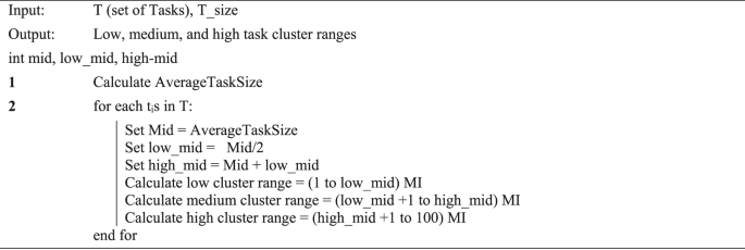 Phase 2: VM clustering
The set of VMs (V) is taken as input by the VM Clustering algorithm and separates V into three different clusters as presented in Algorithm 2 below:
Algorithm 2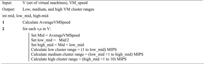 Phase 3: task to VM mapping
The algorithm maps the tasks to the suitable VMs in the corresponding task and VM cluster. The algorithm works in two steps. In step 1, fresh VMs are allocated, and in step 2, the VMs with the minimum ready time are allocated to the next tasks. Algorithm 3 is presented below:
Algorithm 3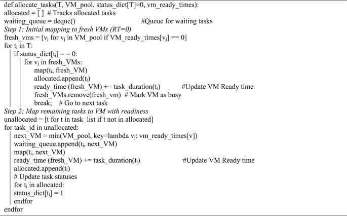
Task to VM mapping without reservation.
Note 1: The Initial task to the VM mapping algorithm maps tasks to VMs without reservation. The algorithm considers all available VMs for allocation created in clustering.
Phase 4: failure modelling and detection via heartbeat mechanism
The set of VMs is taken, and this algorithm tracks every VM for its breaths to detect faulty VMs and is presented in Algorithm 4 below:
Algorithm 4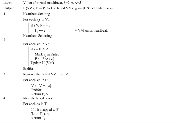 Phase 5: fault tolerance via reservation
The model uses this algorithm in case of a fault in any of the VMs. If any VM fails, the fault tolerance algorithm provides an alternative VM for the affected task based on the reservation. The model uses a structured data structure known as ARM (Advanced Reservation Matrix), used to keep track of the advance reservation task status in the fault tolerance phase. Each row of ARM indicates a particular task to VM reservation and includes the following:
T_ID(\(\:{t}_{i}\)): Unique identifier of the task
VM_ID \(\:{(v}_{f})\): The initially mapped failed VM
VM_ID \(\:{(v}_{j}\)): The reserved VM.
AR_Slot: The advance reservation slot
Status: A flag signifying the state of the reservation
This algorithm is shown below:
Algorithm 5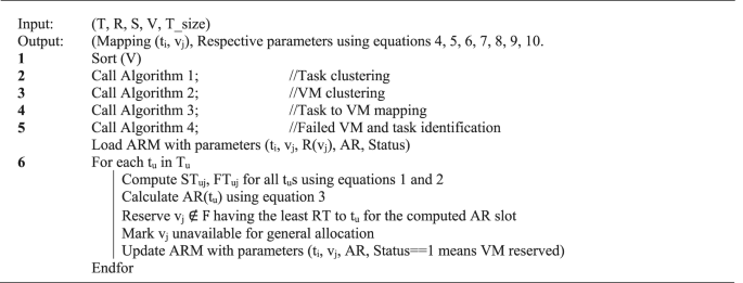
Mapping and fault tolerance algorithm using reservation.
Note 2: When a failed VM and corresponding failed tasks are detected by Algorithm 3, CRFTS reserves the VM with the least ready time entirely for the failed task. This VM is then not considered for general task allocations until the failed task is executed completely.
Figure 3 presents the proposed CRFTS algorithm’s flowchart to aid in understanding the model more clearly. The flowchart includes a detailed representation of the entire procedure.
Fig. 3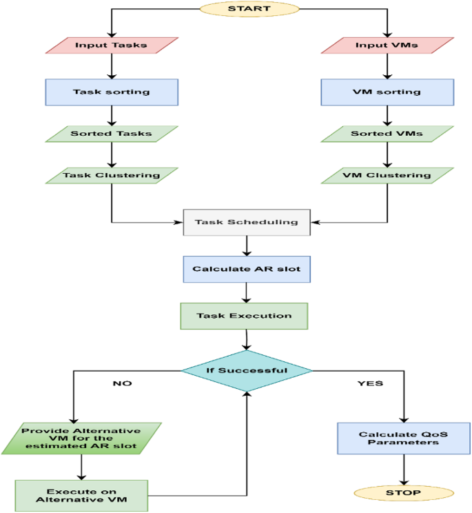 Computational time complexity of CRFTS
CRFTS involves the following Steps:
-
1.
Initialization and Input Parsing
This typically consists of getting the task and VM information. The complexity is O(1) for each input.
Task to VM Mapping
-
2.
Sorting Tasks or VMs:
The algorithm involves sorting tasks or VMs based on Task size and VM Speed. Sorting can be done with the complexity of O(nlogn) and O(klogk), respectively, where n and k are the number of tasks and number of VMs, respectively.
-
3.
Clustering:
Task and VM clusters are obtained with the complexity of O(n) and O(k), respectively. Therefore, the overall complexity of the clustering phase will be O(n+k).
-
4.
Allocating Tasks to VMs within Clusters:
We need to analyze the phases involved in the allocation process. Mapping each task to the VM in the corresponding VM cluster, the complexity can be computed as follows:
Reading the task and VM data:
The complexity will be O(1)
Iterating through task and VM clusters:
We need to iterate through each task cluster to assign tasks to VMs within the corresponding VM cluster. Since there are 3 clusters, let each cluster contain a maximum of m tasks and v VMs, respectively. The complexity of this phase will be O(m+v).
Allocating Tasks to VMs within Clusters:
For each task in a cluster, we allocate it to a VM in the corresponding VM cluster. This typically involves:
-
Iterating through each task in a task cluster: O(m).
-
Iterating through each VM in VM cluster: O(v).
-
Since allocation is performed on two conditions. Therefore, as per the algorithm, the complexity of allocation will be O(1) for the first condition. O(v) for the second condition.
-
The combined complexity will be computed as: O(m) + O(v)+ O(1) +O (v) = O(m+v).
Fault Tolerance Algorithm
The fault tolerance mechanism involves the following steps:
-
-
5.
Detection of faulty VMs:
Checking the status of each VM to detect faults. This step involves iterating through all VMs and can be done in O(k).
-
6.
Redistributing tasks from faulty VMs to healthy VMs:
For f faulty VMs with a maximum of t tasks, the complexity will be O(f⋅t). In the worst case, f⋅t will be equal to n, so the complexity will be O(n).
-
7.
Updating execution times:
Updating the total execution times for VMs. The worst-case complexity will be O(f.t)= O(n).
Combined Total Complexity
Combining these complexities, the overall complexity of CRFTS is dominated by the sorting phase. Thus, the overall time complexity can be expressed as:
O(1) + O(nlogn) + O(klogk) + O(n+k) + O(1) + O(m+v) + O(m) + O(v) + O(1) + O(v) + O(m+v) + O(k) + O(n) + O(n).
=(nlogn) + O(klogk)
Since n will always be greater than k, the final complexity of CRFTS will be O(nlogn).