Friedel oscillations and chiral superconductivity in monolayer NbSe2

We consider the low-energy Hamiltonian for the metallic bands of monolayer NbSe2

$$\hat{H}={\sum} _{{{\bf{k}}},\sigma }{\xi }_{{{\bf{k}}},\sigma }{\hat{c}}_{{{\bf{k}}},\sigma }^{{\dagger} }{\hat{c}}_{{{\bf{k}}},\sigma }+\hat{V},$$

(7)

where the first term describes independent Bloch electrons in the bands crossing the Fermi level with energies ξk,σ, and \({\hat{c}}_{{{\bf{k}}},\sigma }^{({\dagger} )}\) are the creation and annihilation operators of Bloch electrons with crystal momentum k. The second term is the statically screened Coulomb interaction which, in the position representation (1 ≡ r, σ), is defined by a Dyson equation for its matrix elements \(V(1,2)=\left\langle (1,2)\right\vert \hat{V}\left\vert (1,2)\right\rangle\) as

$$V(1,2)={V}_{0}(1,2)+\int\,d(3,4){V}_{0}(1,3)P(3,4)V(4,2),$$

(8)

with V0(1, 2) the matrix elements of the unscreened interaction and P the polarisability of the interacting system. We consider a trigonal 2D lattice with periodic boundary conditions composed of N prismatic unit cells of area Ω and height L with sample volume \({{\mathcal{V}}}=N\Omega L\). The derivation of Eq. (2) from Eq. (8) can be found in the Supplementary Material.

We treat the screening at the RPA level, where the full polarisability in Eq. (8) is replaced with the non-interacting polarisability tensor given by Eq. (4) where

$${\chi }_{\sigma }({{\bf{p}}}+{{\bf{q}}},{{\bf{p}}};\omega )=\frac{1}{N\Omega }\frac{f({\xi }_{{{\bf{p}}}+{{\bf{q}}},\sigma })-f({\xi }_{{{\bf{p}}},\sigma })}{\omega+{\xi }_{{{\bf{p}}}+{{\bf{q}}},\sigma }-{\xi }_{{{\bf{p}}},\sigma }+i\eta },$$

(9)

f is the Fermi function evaluated from the chemical potential μ and the overlaps \({{\mathcal{F}}}\) are defined in Eq. (5). For momenta \({{\bf{k}}}/{{{\bf{k}}}}^{{\prime} }\) outside the first Brillouin zone, Eq. (5) is modified by decomposing \({{\bf{k}}}={{\mathcal{P}}}({{\bf{k}}})+{{\mathcal{Q}}}({{\bf{k}}})\) (see Supplementary Fig. 3), where \({{\mathcal{P}}}\) projects onto the reciprocal lattice, \({{\mathcal{Q}}}\) projects onto the associated crystal momentum and using \({{{\bf{u}}}}_{{{\bf{k}}},\sigma }({{\bf{r}}})={e}^{i{{\mathcal{P}}}({{\bf{k}}})\cdot r}{{{\bf{u}}}}_{{{\mathcal{Q}}}({{\bf{k}}}),\sigma }({{\bf{r}}})\). We express the interaction \(\hat{V}\) entering Eq. (7) in the Bloch basis. It holds for the statically screened Coulomb interaction between Bloch states (see the Supplementary Material for the full derivation),

$$ \left\langle {{\mathcal{Q}}}({{\bf{k}}}+{{\bf{q}}}),\sigma ;{{\mathcal{Q}}}({{{\bf{k}}}}^{{\prime} }-{{\bf{q}}}),{\sigma }^{{\prime} }\right\vert \hat{V}\left\vert {{\bf{k}}},\sigma ;{{{\bf{k}}}}^{{\prime} },{\sigma }^{{\prime} }\right\rangle=\\ \frac{1}{N\Omega }{\sum} _{{{\bf{G}}},{{{\bf{G}}}}^{{\prime} }}{V}_{{{\bf{G}}},{{{\bf{G}}}}^{{\prime} }}^{2{{\rm{D}}},{{\rm{RPA}}}}({{\bf{q}}};{0}^{+}){{{\mathcal{F}}}}_{{{\bf{k}}}+{{\bf{q}}},{{\bf{k}}}}^{\sigma }(-{{\bf{G}}}){{{\mathcal{F}}}}_{{{{\bf{k}}}}^{{\prime} }-{{\bf{q}}},{{{\bf{k}}}}^{{\prime} }}^{{\sigma }^{{\prime} }}({{{\bf{G}}}}^{{\prime} }),$$

(10)

where \({{\bf{k}}},{{{\bf{k}}}}^{{\prime} }\) and q are in-plane momenta restricted to the first Brillouin zone. Noting that the dominant contribution to the matrix element is due to the first few nearest-neighbour sites (see Supplementary Section II D for a discussion) we introduce an effective interaction potential

$$ \left\langle {{\mathcal{Q}}}({{\bf{k}}}+{{\bf{q}}}),\sigma ;{{\mathcal{Q}}}({{{\bf{k}}}}^{{\prime} }-{{\bf{q}}}),{\sigma }^{{\prime} }\right\vert \hat{V}\left\vert {{\bf{k}}},\sigma ;{{{\bf{k}}}}^{{\prime} },{\sigma }^{{\prime} }\right\rangle=\\ \approx \frac{1}{N\Omega }\left({\sum} _{{{\bf{G}}},{{{\bf{G}}}}^{{\prime} }}{V}_{{{\bf{G}}},{{{\bf{G}}}}^{{\prime} }}^{2{{\rm{D}}},{{\rm{RPA}}}}({{\bf{q}}})\right){{{\mathcal{F}}}}_{{{\bf{k}}}+{{\bf{q}}},{{\bf{k}}}}^{\sigma }({{\bf{0}}}){{{\mathcal{F}}}}_{{{{\bf{k}}}}^{{\prime} }-{{\bf{q}}},{{{\bf{k}}}}^{{\prime} }}^{{\sigma }^{{\prime} }}({{{\bf{0}}}}^{{\prime} })\\ =:\frac{1}{N\Omega }{V}^{{{\rm{RPA}}}}({{\bf{q}}}){{{\mathcal{F}}}}_{{{\bf{k}}}+{{\bf{q}}},{{\bf{k}}}}^{\sigma }({{\bf{0}}}){{{\mathcal{F}}}}_{{{{\bf{k}}}}^{{\prime} }-{{\bf{q}}},{{{\bf{k}}}}^{{\prime} }}^{{\sigma }^{{\prime} }}({{{\bf{0}}}}^{{\prime} }),$$

(11)

where we restrict \({{\bf{G}}},{{{\bf{G}}}}^{{\prime} }\) to the range where \({{\mathcal{F}}}({{\bf{G}}})\approx {{\mathcal{F}}}({{\bf{0}}})\) holds, i.e., up to third nearest neighbouring Brillouin zones. This effective interaction potential enables a discussion of the screened interaction on the lattice in terms of a simple q-dependent quantity shown in Fig. 2, but is not used for the calculation of the pairing, where we keep the dependence of the Bloch factors \({{\mathcal{F}}}\) on G.

To access the possible superconducting instabilities described by Eq. (6), we solve a linearised form of the gap equation. First, we project the gap equations on the Fermi surfaces by introducing a local density of states ρk,σ along the Fermi surfaces. We restrict the allowed momenta \({{{\bf{k}}}}^{{\prime} }\) in Eq. (6) to a range around the Fermi surfaces given by a cutoff  ± Λ in energy. Next, we convert the sum over the transverse component \({{{\bf{k}}}}^{{\prime} }-{{{\bf{k}}}}_{{{\rm{F}}}}\) into an integral in energy over this range [ − Λ, Λ]. Assuming that the gap and the interaction vary slowly in this thin shell around each Fermi surface, we can approximate \({\Delta }_{{{{\bf{k}}}}^{{\prime} },\sigma }\approx {\Delta }_{{{{\bf{k}}}}_{{{\rm{F}}}},\sigma }\) and \({V}_{{{\bf{k}}},{{{\bf{k}}}}^{{\prime} },\sigma }\approx {V}_{{{\bf{k}}},{{{\bf{k}}}}_{{{\rm{F}}}},\sigma }\). The resulting gap equation with \({{\bf{k}}},{{{\bf{k}}}}^{{\prime} }\) on the Fermi surfaces takes the form

$${\Delta }_{{{\bf{k}}},\sigma }=-{\sum} _{{{{\bf{k}}}}^{{\prime} }\in {{\rm{FS}}}}{V}_{{{\bf{k}}},{{{\bf{k}}}}^{{\prime} },\sigma }\int_{-\Lambda }^{\Lambda }d\xi {\rho }_{{{{\bf{k}}}}^{{\prime} },\sigma }(\xi )\Pi ({E}_{{{{\bf{k}}}}^{{\prime} }\sigma }){\Delta }_{{{{\bf{k}}}}^{{\prime} },\sigma },$$

(12)

with the pairing function \(\Pi (E)=\tanh (\beta E/2)/2E\). Close to Tc we have Π(E) ≈ Π(ξ) and Eq. (12) becomes a set of linear equations. Instead of starting from the statically screened interaction and applying the mean-field approximation, an alternative approach to the problem is provided by investigating the pair-scattering vertex where the problem also simplifies to the real and static part of the effective pairing interaction18,55. The problem of finding the shape of the order parameter along the Fermi surfaces is equivalent to determining the kernel of a matrix \({{\mathbb{M}}}_{\sigma }\), whose indices are the momenta kF on the Fermi surface, as

$${{\mathbb{M}}}_{\sigma }{{{\mathbf{\Delta }}}}_{\sigma }=0,$$

(13)

where, \(\forall {{\bf{k}}},{{{\bf{k}}}}^{{\prime} }\in {{\rm{FS}}}\),

$${({{\mathbb{M}}}_{\sigma })}_{{{\bf{k}}},{{{\bf{k}}}}^{{\prime} }}={\delta }_{{{\bf{k}}},{{{\bf{k}}}}^{{\prime} }}+{V}_{{{\bf{k}}},{{{\bf{k}}}}^{{\prime} },\sigma }{\rho }_{{{{\bf{k}}}}^{{\prime} },\sigma }{\alpha }^{0}(T,\Lambda ),$$

(14)

$${\alpha }^{0}(T,\Lambda )=\int_{0}^{\Lambda }d\xi \frac{\tanh (\beta \xi /2)}{\xi }.$$

(15)

Here, we assumed a flat density of states ρk,↑(ξ) ≈ ρk,↑ within the energy range  ± Λ around the chemical potential. We rewrite \({{\mathbb{M}}}_{\sigma }\) by factoring out the energy integral α0 in the second summand as

$${{\mathbb{M}}}_{\sigma }={\mathbb{1}}+{\alpha }^{0}(T,\Lambda ){{\mathbb{U}}}_{\sigma },$$

(16)

where \({{\mathbb{U}}}_{\sigma }\) is the pairing matrix containing the interaction and local density of states along the Fermi surfaces. The possible superconducting pairings solving Eq. (13) are the eigenvectors of \({{\mathbb{U}}}_{\uparrow }\) with the corresponding eigenvalues λi fulfilling

$${\lambda }_{i}=-1/{\alpha }^{0}({T}_{{{\rm{c}}},i},\Lambda ),$$

(17)

and Tc,i the critical temperature of the respective instability. The cutoff Λ sets an energy scale against which to measure the gaps and Tc, similar to the Debye frequency in the usual BCS-theory1. In general, not all eigenvectors of \({{\mathbb{U}}}_{\sigma }\) found in this way correspond to physically stable situations67. Similarly, the requirement of vanishing Δk,σ close to Tc,i is only fulfilled if no other superconducting phase with higher Tc is present. As such, we expect only the solution with the highest Tc to be realised. Due to the monotonic nature of α0(T, Λ) as a function of both T and Λ, the solution with the highest critical temperature always corresponds to the lowest negative eigenvalue λ of the pairing matrix. As Λ is a model parameter, we classify and discuss the strength of the different instabilities by their eigenvalues λi.

To investigate how the gaps evolve at temperatures below Tc, we solve Eq. (12) without linearizing. Since we want to use the approximations \({\Delta }_{{{{\bf{k}}}}^{{\prime} },\sigma }\approx {\Delta }_{{{{\bf{k}}}}_{{{\rm{F}}}},\sigma }\) and \({V}_{{{\bf{k}}},{{{\bf{k}}}}^{{\prime} },\sigma }\approx {V}_{{{\bf{k}}},{{{\bf{k}}}}_{{{\rm{F}}}},\sigma }\), we fix the cutoff to the value of Λ = 0.1 eV which, together with the rescaling of the screened interaction to \({\hat{V}}_{\gamma }:=\gamma \hat{V}\) as discussed in the main text, yields Tc = 2 K. This enables us to fit to the experimental Tc while retaining the shape of the interaction as found from our calculation of the screened Coulomb interaction. Since the macroscopic polarisability P0,0 calculated from DFT (see Supplementary Section I B) is even lower at intermediate momentum transfers than our results from a tight-binding calculation, it is plausible that the screened interaction in absence of the substrate is even stronger than our \(\hat{V}\). This is to be expected, since the inclusion of the Se p-orbitals, which contribute most noticeably near the M points, would further diminish the overlaps between states on the Fermi surface, resulting in lower screening.

We expand the gap for one spin species in terms of a restricted set of basis functions, corresponding to the irreducible representations of the symmetry group D3h, as

$${\forall }_{{{\bf{k}}}\in \pi }:\quad {\Delta }_{{{\bf{k}}},\uparrow }={\sum} _{\mu }{f}_{\mu }^{\pi }({{\bf{k}}}){\Delta }_{\mu }^{\pi },$$

(18)

where μ labels basis functions and π ∈ {Γ, K} the Fermi surfaces22,43. We orthonormalise our basis functions with respect to the number Nπ of momenta on each Fermi surface π to satisfy

$${\left\langle {f}_{\mu }^{\pi },{f}_{{\mu }^{{\prime} }}^{\pi }\right\rangle }_{\pi }:=\frac{1}{{N}_{\pi }}{\sum} _{{{\bf{k}}}\in \pi }{f}_{{\mu }^{{\prime} }}^{\pi }({{\bf{k}}})\;{f}_{\mu }^{\pi }({{\bf{k}}})={\delta }_{\mu,{\mu }^{{\prime} }}.$$

(19)

Using this orthogonality, we reduce the dimensionality of the self-consistency problem drastically by projecting the gap equation into a form that couples only the expansion coefficients \({\Delta }_{\mu }^{\pi }\)22. It reads

$${\Delta }_{\mu }^{\pi }=-\frac{1}{{N}_{\pi }}{\sum} _{{\pi }^{{\prime} },{\mu }^{{\prime} }}{\sum} _{\begin{array}{c}{{\bf{k}}}\in \pi \\ {{{\bf{k}}}}^{{\prime} }\in {\pi }^{{\prime} }\end{array}}{f}_{\mu }^{\pi }({{\bf{k}}}){V}_{{{\bf{k}}},{{{\bf{k}}}}^{{\prime} },\uparrow }\,{\rho }_{{{{\bf{k}}}}^{{\prime} },\uparrow }\,{\alpha }_{{{{\bf{k}}}}^{{\prime} }}^{{\pi }^{{\prime} }}\,{f}_{{\mu }^{{\prime} }}^{{\pi }^{{\prime} }}({{{\bf{k}}}}^{{\prime} }){\Delta }_{{\mu }^{{\prime} }}^{{\pi }^{{\prime} }},$$

(20)

where the pairing strength \({\alpha }_{{{\bf{k}}}}^{\pi }\) is given by

$${\alpha }_{{{\bf{k}}}}^{\pi }=\int_{0}^{\Lambda }d\xi \,\frac{\tanh (\beta E(\xi,{\Delta }_{{{\bf{k}}}}^{\pi })/2)}{E(\xi,{\Delta }_{{{\bf{k}}}}^{\pi })}.$$

(21)

At Tc, the pairing strength \({\alpha }_{{{\bf{k}}}}^{\pi }\) becomes independent of k and π. In this case, the orthogonality Eq. (19) yields a linearised gap equation for the expansion coefficients

$${\Delta }_{\mu }^{\pi }=-{\alpha }^{0}{\sum} _{{\pi }^{{\prime} },{\mu }^{{\prime} }}{U}_{\mu,{\mu }^{{\prime} }}^{\pi,{\pi }^{{\prime} }}{\Delta }_{\mu }^{{\pi }^{{\prime} }},$$

(22)

where the pairing matrix \({\mathbb{U}}\) in this representation is given by

$${U}_{\mu,{\mu }^{{\prime} }}^{\pi,{\pi }^{{\prime} }}=\frac{1}{{N}_{\pi }}{\sum} _{{{\bf{k}}}\in \pi,{{{\bf{k}}}}^{{\prime} }\in {\pi }^{{\prime} }}{f}_{\mu }^{\pi }({{\bf{k}}}){V}_{{{\bf{k}}},{{{\bf{k}}}}^{{\prime} },\uparrow }\,{\rho }_{{{{\bf{k}}}}^{{\prime} },\uparrow }{f}_{{\mu }^{{\prime} }}^{{\pi }^{{\prime} }}({{{\bf{k}}}}^{{\prime} }).$$

(23)

To account for the mixing between different symmetries due to the k dependence of \({\alpha }_{{{\bf{k}}}}^{\pi }\) below Tc, we insert a unity in Eq. (20) to arrive at

$${\Delta }_{\mu }^{\pi }=-{\sum} _{{\pi }^{{\prime} },{\mu }^{{\prime} },{\mu }^{{\prime\prime} }}{U}_{\mu,{\mu }^{{\prime} }}^{\pi,{\pi }^{{\prime} }}{\Upsilon }_{{\mu }^{{\prime} },{\mu }^{{\prime\prime} }}^{{\pi }^{{\prime} }}{\Delta }_{{\mu }^{{\prime\prime} }}^{{\pi }^{{\prime} }},$$

(24)

where the mixing of different basis functions is described by

$${\Upsilon }_{\mu,{\mu }^{{\prime} }}^{\pi }=\frac{1}{{N}_{\pi }}{\sum} _{{{\bf{k}}}\in \pi }{f}_{\mu }^{\pi }({{\bf{k}}}){\alpha }_{{{\bf{k}}}}^{\pi }{f}_{{\mu }^{{\prime} }}^{\pi }({{\bf{k}}}).$$

(25)

For an incomplete set of basis functions this insertion of unity becomes approximate, but in our case still suffices to capture the weak mixing between basis functions induced by \({\alpha }_{{{\bf{k}}}}^{\pi }\). As such, we employ Eq. (24) to numerically determine the evolution of the solutions obtained from the linearised equations below their Tc,i. The basis functions we used and the temperature dependence curves for the respective expansion coefficients are shown in Supplementary Section III A.

We define a purely chiral solution as

$${\Delta }_{{{\rm{p}}}+{{\rm{ip}}}}=\frac{| | {\Delta }_{{{\rm{py}}}}| | }{| | {\Delta }_{{{\rm{px}}}}| | }{\Delta }_{{{\rm{px}}}}+i{\Delta }_{{{\rm{py}}}},$$

(26)

where \(| | \Delta | | :=\sqrt{{\sum }_{\pi=G,K}{\langle \Delta,\Delta \rangle }_{\pi }}\), with the scalar product defined in Eq. (19). The Δpx component is renormalised so that both nematic solutions enter with the same weight. The ratio of admixture Rch of Δp+ip in the chiral solution Δch in Fig. 4a is defined as

$${R}_{{{\rm{ch}}}}:=\frac{| {\sum}_{\pi=\Gamma,K}{\langle {\Delta }_{{{\rm{p}}}+{{\rm{ip}}}},{\Delta }_{{{\rm{ch}}}}\rangle }_{\pi }| }{| | {\Delta }_{{{\rm{ch}}}}| | \,| | {\Delta }_{{{\rm{p}}}+{{\rm{ip}}}}| | }.$$

(27)

The square root of mean squared Δ shown in Fig. 4a for each gap symmetry is \(\sqrt{\langle {\Delta }^{2}\rangle }\equiv | | \Delta | |\).

The free energy of a superconductor with gap Δkσ can be written as

$$F=\frac{1}{2}{\sum} _{{{\bf{k}}}\sigma }\left({\xi }_{{{\bf{k}}}\sigma }-{E}_{{{\bf{k}}}\sigma }+\Pi ({E}_{{{\bf{k}}}\sigma })| {\Delta }_{{{\bf{k}}}\sigma }{| }^{2}\right)\\ -{k}_{TB}T{\sum} _{{{\bf{k}}}\sigma }{{\rm{In}}} \left(1+{e}^{-{E}_{{{\bf{k}}}\sigma }/{k}_{TB}T}\right).$$

(28)

Note that this free energy is written assuming that the gap obeys the self-consistent equations (see Supplementary Section III). It cannot be used to find the physical gaps by minimization with respect to Δkσ, but does yield the correct result once a solution is found by solving the self-consistent gap equations67. We therefore use it to rank the solutions by their free energy gain within the energy window of  ± 2 meV where the contributions of different gap symmetries are distinguishable.

NbSe2 monolayers2 were grown on graphitised (bilayer graphene) on 6H-SiC(0001) by molecular beam epitaxy (MBE) at a base pressure of ~ 2 ⋅ 10−10 mbar in our home-made ultrahigh-vacuum (UHV) MBE system. SiC wafers with resistivities ρ ~120 Ωcm were used68.

Reflective high-energy electron diffraction (RHEED) was used to monitor the growth of the NbSe layer2. During the growth, the bilayer graphene/SiC substrate was kept at 580 °C. High-purity Nb (99.99%) and Se (99.999%) were evaporated using an electron beam evaporator and a standard Knudsen cell, respectively. The Nb:Se flux ratio was kept at 1:30, while evaporating Se led to a pressure of ~ 5 ⋅ 10−9 mbar (Se atmosphere). Samples were prepared using an evaporation time of \(30\,\min\) to obtain a coverage of  ~ 1 ML. To minimise the presence of atomic defects, the evaporation of Se was subsequently kept for an additional 5 minutes. Atomic force microscopy (AFM) under ambient conditions was routinely used to optimise the morphology of the NbSe2 layers. The samples used for AFM characterization were not further used for the scanning tunnelling microscope (STM). Lastly, to transfer the samples from our UHV-MBE chamber to our STM, they were capped with a  ~10 nm amorphous film of Se, which was subsequently removed by annealing at the STM under UHV conditions at 280 °C.

Scanning tunnelling microscopy/spectroscopy experiments were carried out in a commercial low-temperature, high magnetic field (11 T) UHV-STM from Unisoku (model USM1300) operated at T = 0.34 K unless otherwise stated. STS measurements (using Pt/Ir tips) were performed using the lock-in technique with typical ac modulations of 20–40 μV at 833 Hz. All data were analyzed and rendered using WSxM software69. To avoid tip artifacts in our STS measurements, the STM tips used for our experiments were previously calibrated on a Cu(111) surface. A tip was considered calibrated only when tunnelling spectroscopy performed on Cu(111) showed a sharp surface state onset at  −0.44 eV followed by a clean and monotonic decay of the differential conductance signal (i.e., dI/dV). In addition to this, we also inspected the differential conductance within  ±10 mV to avoid strong variations around the Fermi energy.

For spectroscopy in the tunnelling regime with a normal metal tip, the differential conductance is given by

$$G(V)={\sum}_{{{\bf{k}}},\sigma }{C}_{{{\bf{k}}}\sigma }\int_{-\infty }^{\infty }\frac{{{\rm{d}}}E}{2\pi }\,{A}_{{{\rm{s}}}}({{\bf{k}}},\sigma ;E)\left(-\frac{\partial f(E+eV)}{\partial E}\right),$$

(29)

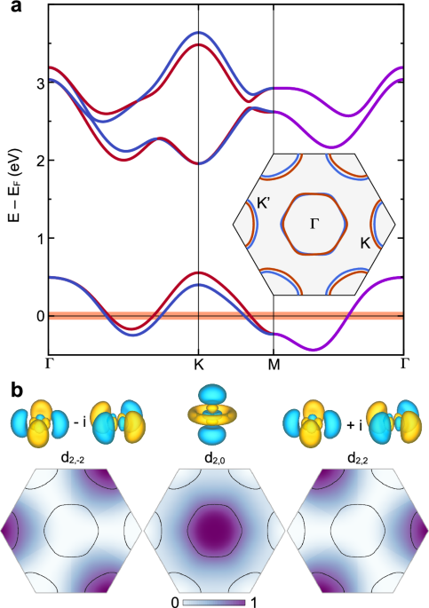
where As is the spectral function of the superconductor. The coupling Ckσ accounts for the spectral function of the tip and the tunnelling overlap between the tip’s evanescent states and quasiparticle states from the superconductor with momentum k and spin σ. We do not expect the coupling to vary much on any given Fermi surface π, and as such we approximate Ck,σ ≈ Cπ. However, due to the different orbital composition and in-plane momenta of the quasiparticle states at the K, \({K}^{{\prime} }\) valleys and at the Γ surface, cf. Fig. 1b, the coupling constant will be in general different. In particular, since the d2,0 orbital extends farthest out of plane and the STM favours states with small in-plane momentum63, as has been observed in previous STM measurements32, we expect CΓ ≫ CK.

In the tunnelling regime, where the experimental data was taken, the lifetime of the quasiparticles is weakly affected by the coupling to the tip and the spectral function can be approximated with the local density of states of the quasiparticles, As(k, σ, E) = 2πDk,σ(E). The tunnelling to each of the Fermi surfaces represents a distinct transport channel, whose strength is given by the sum over the local density of states

$${D}_{\pi,\sigma }(E)={\sum}_{{{\bf{k}}}\in \pi }{D}_{{{\bf{k}}},\sigma }(E).$$

(30)

The latter are modeled by assuming a BCS form factor modifying the local density of states ρk,σ in the normal conducting state as

$${D}_{{{\bf{k}}},\sigma }(E)={\rho }_{{{\bf{k}}},\sigma }{{\rm{Re}}}\sqrt{\frac{{E}^{2}}{{E}^{2}-| {\Delta }_{{{\bf{k}}},\sigma }{| }^{2}}}.$$

(31)

In the absence of magnetic fields, we can assume that, due to time reversal symmetry, Dπ,σ = Dπ/2 and Cπ,σ = Cπ. As such, Eq. (29) predicts for the total differential conductance a superposition of contributions from the distinct transport channels with weights provided by the couplings Cπ as

$$G(V)\approx {\sum}_{\pi }{C}_{\pi }{G}_{\pi }(V),$$

(32)

$${G}_{\pi }(V)=\int_{-\infty }^{\infty }{{\rm{d}}}E\,{D}_{\pi }(E)\left(-\frac{\partial f(E+eV)}{\partial E}\right).$$

(33)

For low temperature, the form of the gap on each separate Fermi surface results in characteristic signatures in the differential conductance of the respective transport channel. We use as a fit function this superposition of the differential conductance of the individual transport channels. For the gaps on the Fermi surfaces Δk,σ, we use the form of the gaps as found from Eq. (24) at the experimental temperature \({T}_{\exp }\) indicated by stars in Fig. 4a. For single-band s-wave superconductors the ratio between the amplitude of the gap and the critical temperature is fixed as \(\Delta (T=0\,{{\rm{K}}})/({k}_{{{\rm{B}}}}{T}_{{{\rm{c}}}})=\pi {e}^{-{\gamma }_{{{\rm{e}}}}}\approx 1.76\), with Euler’s constant γe1. This ratio appears to be slightly violated in monolayer 1H-NbSe2 as the expected s-wave gap for the Tc ≈ 2 K is Δ(T = 0 K) ≈ 0.3 meV instead of the roughly 0.4−0.5 meV gap we find in the spectral function, in agreement with earlier works33. Such violations of the BCS-ratio are known to occur in multi-band or multi-patch superconductors and have been observed previously18,70. To account for this possibility, we allow for a fit of the amplitude of our solution by a common rescaling of all Δk,σ by a parameter A as Δk,σ → AΔk,σ. The latter also takes care of the uncertainty of the actual experimentally realised Tc and the rescaling factor γ of the interaction.

To qualitatively account for additional sources of broadening in the experiment, we fit with an effective temperature Teff in the calculation of the derivative in Eq. (33) which ranges between 1.3 and 1.4 times the recorded base temperature of the STM in Fig. 4d, e and is kept at 1.4 times the measurement temperature for Fig. 4f. To account for offsets in the calibration, we further allow for both a small constant offset G0 in the measured conductivity and V0 in the recorded voltage. The fit coefficients for the other traces shown in Fig. 4d, f only differ by small quantitative changes from the ones reported in Table 1 for Fig. 4e. For the fitting we use the trust region reflective algorithm as implemented in SciPy’s “curve_fit” routine. We consider a range of  ± 0.5 mV containing the main coherence peaks, but not the satellite features due to Leggett modes33, which are not accounted for in our theory. The resulting fit parameters are listed in Table 1. The best fits for the solutions associated with the \({E}^{{\prime} }\) irreducible representation are obtained by considering strongly selective coupling of the tip to the Γ pockets.

Table 1 Fit coefficients for comparison between STS experiment and theory in Fig. 4(e)