Sample preparation
To fabricate the WSe2/PTCDA heterostructure (Extended Data Fig. 1a), hBN was first exfoliated onto a 0.1% niobium-doped SrTiO3 substrate and an approximately 50-nm-thick flake was identified by optical microscopy. In a parallel procedure, WSe2 monolayers were directly exfoliated onto a silicone gel film (DGL Film, Gel-Pak) and identified through optical microscopy and Raman spectroscopy. Afterwards, a monolayer WSe2 flake was transferred from the silicone gel film onto the hBN flake on the SrTiO3 substrate (Extended Data Fig. 1b). After introduction into ultrahigh vacuum (−9 mbar), the sample was annealed at 670 K for 2 h to ensure a clean sample surface. The bare monolayer WSe2 was analysed with the momentum microscope in real space (Extended Data Fig. 1c) and reciprocal space (Extended Data Fig. 2e), showing the expected characteristic features of monolayer WSe2, that is, the spin-split valence bands at the K valley and a single parabolic band at the Γ valley below the global VBM at the K valley (Fig. 1b and refs. 20,23). Moreover, the clear separation between the top and the bottom valence band (Fig. 1c) indicates the high-quality of the WSe2 with only contributions of inhomogeneous broadening.
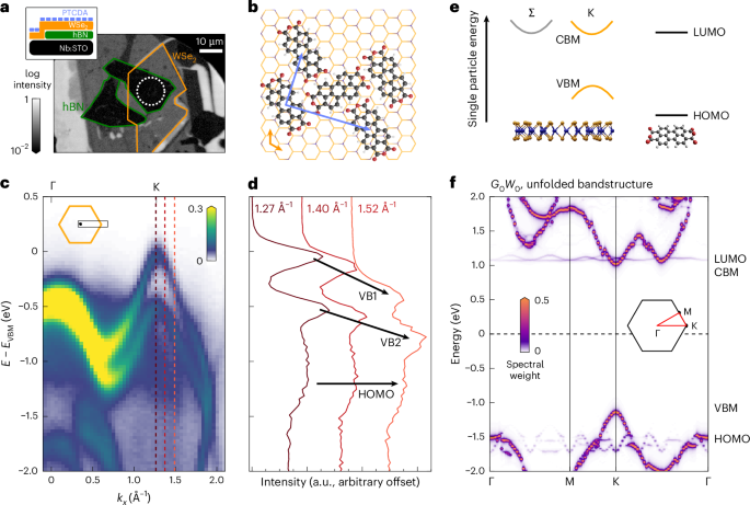
Subsequently, approximately a monolayer of PTCDA was thermally evaporated onto the sample, which was maintained at room temperature (base pressure −9 mbar). The deposition rate was monitored with a with a quartz crystal microbalance and calibrated using the known deposition of PTCDA onto a Ag(110) crystal surface. On the Ag(110) surface, the first monolayer of PTCDA is adsorbed in a brickwall structure whereas additional layers grow in a Herringbone structure with a different superstructure that can be analysed by low energy electron diffraction (LEED)51. By step-wise evaporation of PTCDA onto Ag(110) and recording of the LEED pattern, the evaporation rate was determined and was then used to deposit a monolayer PTCDA onto monolayer WSe2. The successful deposition of a monolayer PTCDA onto monolayer WSe2 was confirmed by the observation of additional spectral weight in the static ARPES data, which can be attributed to the HOMO of PTCDA (Fig. 1c,d) and backfolded WSe2 bands (Extended Data Fig. 1e), which are caused by the adsorbed molecular PTCDA superstructure (Fig. 1b). The superstructure matrix
$$M=\left[\begin{array}{cc}1.58&6.78\\ 4.39&1.32\end{array}\right]$$
was determined by LEED on a cleaved WSe2 bulk crystal (Extended Data Fig. 1d) and is in good agreement with ref. 28 and the ARPES data (Extended Data Fig. 1e).
Femtosecond momentum microscopy
All photoemission data were acquired with the Göttingen in-house photoemission set-up17,52 that combines a time-of-flight momentum microscope53 (Surface Concept GmBH, ToF-MM) with a 500-kHz high-harmonic generation beamline (26.5 eV p-polarized, 20 fs). For the time-resolved measurements, the photon energy of the s-polarized pump was tuned to hν = 1.7 eV with 50 ± 5 fs pulse duration using an optical parametric amplifier. The experimental set-up is described in detail in ref. 17. The pump fluence was adjusted to 280 ± 20 μJ cm−2, which results approximately in an initial K-exciton density of (5.4 ± 1.0) × 1012 cm−2 (refs. 31,48). All experiments are performed with an energy, momentum and time resolution of 200 ± 30 meV, 0.04 ± 0.01 Å−1 and 54 ± 7 fs (refs. 17,31,54). The static measurements (Fig. 1c) were performed at T = 50 K, while all pump–probe delay-dependent measurements were performed at room temperature (300 K).
Photoemission data processing
The time-of-flight momentum microscope enables the simultaneous measurement of the kinetic energy and both in-plane momenta of the photoemitted electrons53. However, the acquired three-dimensional photoemission data are affected by various lens aberrations and other distortions, such as pump- and probe-induced space-charge effects and surface photovoltage55,56,57. Therefore, the photoemission data needs to be preprocessed before further evaluation by (1) correcting a time-dependent rigid energy shift and (2) correcting for distortions that are induced by the projection and focal lens system.
First, the time-dependent energy shift was corrected by minimizing the variance between the momentum-integrated spectra for E − EVBM 58,59. We then determined the parameters for an affine transformation that maps the measured data onto an undistorted and energy-independent grid. This transformation is applied to all datasets. Small remaining distortions induced by the first lens system were corrected by fitting the positions of the K-excitons and mapping them onto an equilateral hexagon. The same positions were used to perform the momentum calibration using the lattice constant of \({{\rm{WSe}}}_{2} \, {a}_{{{\rm{WSe}}}_{2}}=0.3297\,\rm{nm}\). In addition, for each delay step, the data were momentum-wise normalized to the energy range between E − EVBM = −1.8 and −3.8 eV. This momentum-wise normalization accounts for potential changes in illumination due to possible instabilities during the long integration times of the time-resolved measurements.
Quantitative analysis of the exciton energies and dynamics
The EUV laser pulses fragment the Coulomb-bound electron–hole pairs into their single-particle components. As this process conserves energy and momentum33,60,61, the exciton energies Eexc can be extracted by fitting the delay-integrated (100–500 fs), background-substracted (see the non-negative matrix formalism (NMF) method below) and momentum-filtered EDCs shown in Fig. 2c with either one (K- and Σ-excitons) or two (hX) Gaussian peaks Ip and an exponential background Ibg, that is,
$${I}_{{\rm{p}}}(E\;)=\frac{A}{\sigma \sqrt{2\uppi }}\exp \left\{\left(-\frac{{(E-\mu )}^{2}}{2{\sigma }^{2}}\right)\right\},$$
(1)
$${I}_{{\rm{bg}}}(E\;)={A}_{{\rm{bg}}}\exp \left\{\left(-\frac{E}{{\tau }_{{\rm{bg}}}}\right)\right\}.$$
(2)
The extracted peak energies E − EVBM of the K and Σ excitons directly correspond to the exciton energies Eexc because the hole resides at the VBM of WSe2. For the hX, the peak energy of the higher lying peak at E − EVBM = 1.57 ± 0.05 eV directly corresponds to \({{{E}}}_{{\rm{exc}}}^{{\rm{hX}}}\), whereas the lower-energy peak at E − EVBM = 0.38 ± 0.05 eV has to be referenced to the HOMO at E − EVBM = −1.2 ± 0.1 eV, which results in the same exciton energy \({{{E}}}_{{\rm{exc}}}^{{\rm{hX}}}\) = 1.58 ± 0.1 eV. In Extended Data Table 1, the quantified exciton energies \({{{E}}}_{{\rm{exc}}}^{i}\) are compared with the BSE@G0W0 calculations and ARPES and photoluminesence experiments on monolayer WSe2 (refs. 22,23,62). The total error of the experimental values is estimated to be approximately 0.05 eV, taking into account fitting errors and possible errors induced by the energy calibration and space charge effects.
To analyse the exciton dynamics of the K, Σ and hX photoemission signatures (Fig. 5), we filter the raw photoemission data, that is, without background subtraction, by their energy and momentum coordinate. The respective EDCs and the chosen region of interests are shown in Extended Data Fig. 4. To quantify the rise time, we fitted the energy- and momentum-filtered time-resolved photoemission spectral weight traces with an error function
$$I(t)=\frac{1}{2}\left(1+\,\text{erf}\,\left(\frac{t-{\mu }_{{\rm{onset}}}}{\sqrt{2}{\sigma }_{{\rm{rise}}}}\right)\right)$$
(3)
in the delay regions −200 fs to 0 fs, −200 fs to 20 fs and −200 fs to 150 fs, respectively (Extended Data Fig. 6). Here, μonset indicates the onset time, while σrise is directly related to the rise time.
Similarly, we fitted the decay of photoemission spectral weight with a bi-exponential decay (equation (4)) between 0 fs and 2,000 fs and between 20 fs and 2,000 fs for the K- and Σ-excitons, respectively. The hX was fitted with a single exponential decay function (equation (5)) between 200 fs and 2,000 fs:
$$I(t)=A\left(\frac{1}{1+f}\exp \left\{\left(-\frac{t}{{\tau }_{{\rm{fast}}}}\right)\right\}+\frac{f}{1+f}\left(-\frac{x}{{\tau }_{{\rm{slow}}}}\right)\right),$$
(4)
$$I(t)=A\exp \left\{\left(-\frac{t}{{\tau }_{{\rm{slow}}}}\right)\right\}.$$
(5)
The relevant time constants are given in Extended Data Table 1.
Non-negative matrix factorization
Due to the small size of the WSe2 monolayer and the small real-space selection aperture (10 μm effective diameter), the measurement was susceptible to a time-independent background intensity. Therefore, the excited state momentum maps and momentum-filtered EDCs shown in Fig. 2 and in the insets of Extended Data Fig. 4 and 6 were background subtracted.
For the background determination, we used NMF, as implemented in the scikit-learn package for Python63. NMF is a dimensionality-reduction method that so far remains unexplored in time-resolved ARPES, but it has recently found application in spatially resolved material science studies based on X-ray diffraction64 and also static ARPES experiments65. Similar to principal component analysis, NMF is based on the numerical factorization of a given matrix X into two matrices W and H, with the additional condition that all matrices have only non-negative elements. In our case, X is given by the time-dependent raw dataset where we consider only excited state data above E − EVBM = 0.15 eV. In addition, we fix W by a static background and the four extracted time traces of the K, Σ, hX@1.6 eV and hX@0.4 eV photoemission signal plotted in Fig. 5. The determined output then is the matrix H that consists of five components, each following one of the four given time dependencies and the time-independent background. Extended Data Fig. 3 shows extracted components integrated over the regions of interest in energy. Notably, the different components 1–4 can be assigned in reasonable agreement to the different excitonic photoemission signatures despite the strong overlap in time, energy and momentum (orange hexagons, grey circles and blue circle). Component 5 is time-independent and used for background substraction.
Photoemission orbital tomography
Using the plane-wave model of photoemission, the measured momentum-dependent photoemission intensity of electrons emitted from molecular orbital can be expressed as34
$$I({\bf{k}})={\left\vert {\bf{A}}\cdot {\bf{k}}\right\vert }^{2}{\left\vert {\mathscr{F}}\left(\psi ({\bf{r}})\right)\right\vert }^{2}\delta \left({E}_{\rm{b}}+{E}_{{\rm{kin}}}+\varPhi -h\nu \right),$$
(6)
where ψ(r) is the real-space electronic wavefunction, \({\mathscr{F}}\) is the Fourier transform and \({\left\vert {\bf{A}}\cdot {\bf{k}}\right\vert }^{2}\) is a polarization factor defined by the vector potential A of the incoming electromagnetic field. The Dirac δ function ensures energy conservation of the photoemission process, which includes the photon energy hν, the electron binding energy Eb, the work function Φ and the kinetic energy Ekin of the emitted photoelectron. This model has been successfully applied to analyse orbital wavefunctions of transient excited states in PTCDA26 and extended to the description of the photoemission signature of excitons in C60 (ref. 36). According to refs. 36,37, the photoemission signature of the hX with multiple hole contributions, but only a single electron contribution, must feature a two-peak structure, where the momentum distribution of both peaks resembles the Fourier transform of the LUMO of PTCDA as described by equation (6). Based on this model, we calculate the expected momentum map of the HOMO and the hX considering all the different orientations of the PTCDA molecule28. The real-space molecular orbitals calculated by DFT are extracted from ref. 66. The results are plotted in Extended Data Fig. 2c,g. We note that the theoretical momentum fingerprints were calculated for single-particle electrons (that is, using the Kohn–Sham orbitals). In the near future, progress in the field of exciton photoemission orbital tomography36,37 may enable the calculation of predicted momentum fingerprints also for excitonic states; however, such calculations are currently not possible for the present WSe2/PTCDA structure.
Calculation of the electronic structure
A G0W0 treatment of the herringbone-type WSe2/PTCDA heterostructure is beyond current computational possibilities. Instead, to meet the experimental conditions as closely as possible, we consider a configuration of a PTCDA molecule adsorbed on a 4 × 4 × 1 supercell of the pristine WSe2 structure with an in-plane lattice parameter of 3.317 Å (Extended Data Fig. 5; for a detailed discussion of the implemented supercell, refer to the Supplementary Information). We optimize the atomic structure, consisting of 86 atoms, using the all-electron code ‘FHI-aims’67 by minimizing the amplitude of the interatomic forces below a threshold value of 10−3 eV Å−1. For all species a tight basis is used. The resulting adsorption geometry is shown in Extended Data Fig. 5a. The PTCDA molecule is slightly tilted, with the shortest and longest distance to the substrate being 2.87 Å and 4.98 Å, respectively, measured from the top of the substrate.
The ground-state, G0W0 and BSE calculations are performed using the all electron full-potential code ‘exciting’29, which implements the family of linearized augmented plane wave plus local orbitals (LAPW+LO) methods. The muffin-tin spheres of the inorganic component are chosen to have equal radii of 2.2 bohr. For PTCDA, the radii are 0.9 bohr for hydrogen (H), 1.1 bohr for carbon (C) and 1.2 for oxygen (O). The electronic properties are calculated first using DFT with the generalized gradient approximation in the Perdew–Burke–Ernzerhof parametrization for the exchange–correlation (xc) functional. The sampling of the BZ is carried out with a homogeneous 3 × 3 × 1 Monkhorst–Pack k-point grid. To account for van der Waals forces and intermolecular interactions, we adopt the Tkatchenko–Scheffler method68. The quasi-particle (QP) energies are computed within the G0W0 approximation69, where we include 200 empty states to compute the frequency-dependent dielectric screening within the random-phase approximation. A 2D truncation of the Coulomb potential in the out-of-plane direction z is used70. The band structure is computed by using interpolation with maximally localized Wannier functions71 and Fourier interpolation (Extended Data Fig. 5b and Extended Data Fig. 5c, respectively). To keep the calculations feasible, SOC is not considered in this work. Although SOC leads to a splitting of the lowest-energy excitonic peak by approximately 450 meV (ref. 72), it would not alter the type-I level alignment of WSe2/PTCDA. Importantly, the molecular states involved in the formation of the hX, that is, the HOMO and LUMO, would not be affected by the inclusion of SOC.
To allow a direct comparison with the experimental ARPES data (Fig. 1d), we unfold the theoretical band structure by symmetry mapping of the Bloch-vector-dependent quantities defined in the supercell into the unit-cell calculations. Here, the wavefunctions are constructed in a uniform real-space grid of 120 × 120 × 120 and used to calculate the spectral function (Fig. 1f).
The QP band gap of WSe2 in the heterostructure is in good agreement with that measured by STS28; however, the PTCDA gap is underestimated, which is most evident in the level alignment of the HOMO. This discrepancy can be explained by the interplay of different effects such as SOC, the choice of the xc functional and its role as a starting point for the QP calculations, and the interlayer distance between PTCDA and WSe2. Uncertainties in the latter can be related to packing density, the xc functional and the treatment of van der Waals interactions, or temperature73. In earlier studies on ZnO/WSe2 it has been shown that increasing the interlayer distance leads to a noticeable increase in the QP gaps on both sides of the interface74. Also in WSe2/PTCDA, increasing (decreasing) the interlayer distance will decrease (increase) the mutual screening, leading to an increase (decrease) in the HOMO–LUMO gap. This, in turn, would lead to an increase (decrease) in the VBM–HOMO distance. Overall, there is an interplay of effects on the order of a few tenths of an electronvolt each, which can only be resolved through extensive future QP calculations.
To overcome this mismatch, we apply a scissors shift to the molecular levels. Shifting the LUMO by −50 meV closer to the experimental value28 results in very good agreement of the excitonic spectrum with experiment (see below).
Calculation of the exciton spectrum
For the calculation of the exciton spectrum, we solve the BSE on top of the QP band structure, where the screened Coulomb potential is computed using 100 empty bands. In the construction and diagonalization of the BSE Hamiltonian, 16 occupied and 14 unoccupied bands are included, and a 12 × 12 × 1 shifted k-point mesh is adopted. Calculations are performed using the BSE module75 of the ‘exciting’ code.
Calculation of the correlation function
Following the definition in ref. 40, we calculate the electron–hole correlation function
$${F}^{i}(\bf{r})={\int}_{\varOmega }{d}^{\,3}{{\bf{r}}}_{\rm{e}}| {\psi }_{i}({{\bf{r}}}_{\rm{h}}={{\bf{r}}}_{\rm{e}}+{\bf{r}},{{\bf{r}}}_{\rm{e}}){| }^{2},$$
(7)
where Fi describes the probability of finding electron and hole separated by the vector r = rh − re. We approximate this integral by a discrete sum over a finite number of fixed electron coordinates. For each electron position, the hole probability ∣ψi(rh = re + r, re)∣2 is computed on an evenly spaced, dense grid of 100 × 100 × 100 sampling points, covering approximately 3 × 3 × 1 supercells. For the hX, we sampled 60 positions on the PTCDA molecule (0.5 Å−1 below and above the carbon and oxygen atoms) because its electronic contribution is almost entirely composed of the LUMO of PTCDA. Similarly, we calculated the electron–hole correlation function of the K-exciton (Extended Data Fig. 7), which is completely localized in the WSe2 layer. Here, we sampled 16 positions close to the W atoms where we expect a high probability of finding the electron.
For further analysis, the three-dimensional correlation function is split into its in-plane and out-of-plane components by integrating over the other direction (Fig. 4 and Extended Data Fig. 7). Here, the intralayer (purple) and interlayer (green) in-plane distributions were extracted by integrating exclusively over the respective peak of F(r⊥), that is, r⊥ = −3 to 4.5 Å and r⊥ = −10.5 to −3 Å for the intra- and interlayer components, respectively. Notably, the in-plane component shows a distinct periodic pattern (see insets in Fig. 4b and Extended Data Fig. 7b). Thus, to extract the in-plane radial profile and the root mean square (RMS) radius, we first filter the data in Fourier space, thereby smoothing it in the real space.
Spatial analysis of the K-exciton and comparison with hX
In analogy to the analysis of the spatial structure of the hX in Fig. 4, we analyse the K-exciton wavefunction (Extended Data Fig. 7). From the BSE calculation, we find that FK(r⊥) is dominated by a single peaked feature centred around r⊥ ≈ 0 Å, implying that the exciton is of pure intralayer character (Extended Data Fig. 7a). Consequently, the probability density of finding K-excitons in the WSe2 layer is nearly 100%. Consistent with this, the two smaller side peaks located at a distance corresponding to the distance between the tungsten and selenium planes dW,Se, can be attributed to a residual probability of the electron and/or hole being at the selenium atoms.
Due to its hydrogen-like structure, the in-plane electron–hole probability distribution of the K-exciton can be directly reconstructed from the experimental photoemission momentum fingerprint via Fourier analysis31,41,42,59. This allows a direct comparison of FK(r∥) between theory and experiment (Extended Data Fig. 7b). Both theory and experiment confirm the pure Wannier-like character of the K-exciton because the radial distribution is much larger than the WSe2 lattice constant. For a more quantitative analysis, we compare the extracted RMS radii to be (\({{{r}}}_{{\rm{K}}}^{{\rm{BSE}}}\) = 14 Å) (theory) and \({{{r}}}_{{\rm{K}}}^{\exp }\) = 10 ± 1 Å (experiment), which are in excellent agreement. Note that, due to the finite momentum resolution of the photoemission signal, the derived RMS radius represents a lower limit of the true value. The distinct intralayer and Wannier-like character of the K-exciton can be further visualized by plotting the isosurface of a representative fixed electron and hole position (Extended Data Fig. 7c), which stands in clear contrast to the isosurfaces of the hX (Fig. 4).
After having identified the K-exciton as a Wannier exciton, we compare its in-plane correlation function directly to that of the inter- and intralayer contributions to the hX (Extended Data Fig. 8). Here, we find that the interlayer contribution resembles the spatial distribution of the K-exciton, while the intralayer contribution is more localized and exhibits a stronger spatial modulation stemming from the molecular orbitals. This direct comparison confirms the previously assigned Frenkel- or Wannier-type character of the intra- and interlayer contribution of the hX.
For comparison, the calculated RMS radii of the K-exciton and both components of the hX are summarized in Extended Data Table 2.