Ethics
Both waves of data collection (see below) were approved by the Regional Ethical Review Board in Stockholm (Dnrs 2011/570-31/5, 2012/1107/32, 2021-02014, 2022-00109-02, 2020-02575). All methods and procedures followed international guidelines in accordance with the Declaration of Helsinki.
SampleSwedish Twin Registry: Screening Twin Adults Genes and Environment (STAGE)
Participants were twins recruited from the Swedish Twin Registry71. Twin zygosity was determined by questionnaire data, which, when compared to genotypes, has been shown to be 99% accurate in the Swedish Twin Registry72. The twins included in this study took part in two large recent waves of online data collection on music, art, and cultural engagement. In 2011 and then again in 2022, a total of 32,005 adult twin individuals were invited from the STAGE cohort born between 1959 and 1985, of which around 11,500 participated in the first wave and then around 9500 in the latest wave. In the first wave of data collection, participants completed the Swedish Musical Discrimination Test (see below). More details on this wave can be found in Ullén et al.12. Additionally, in the second wave, the Behavioral Approach System39 and Barcelona Music Reward Questionnaire10 were administered. We note that response rates in the STAGE cohort have been low (~30%). The low response rates presumably reflect that this is a population-based study (i.e., where a whole birth cohort of Swedish twins is invited to participate) of a working-aged cohort; this is a general phenomenon not unique to our study71. A full description of the twin sample across waves of data collection can be found in Table 1, including n of twins for which we had both data available, stratified by the zygosity and the sex of the twins; for both waves of data collection, informed consent was given by each participant before data gathering began.
Primary measureBarcelona Music Reward Questionnaire (BMRQ)
The Barcelona Music Reward Questionnaire (BMRQ) is a psychometric tool used to assess musical anhedonia11,15 and, more generally, music reward sensitivity10, which has previously been validated across many cultures10,68,69,70. It comprises 20 self-report items, with five response options, ranging from completely disagree to completely agree. After recoding response items to numeric options (1–5), with two out of 20 items being reverse coded, we used the sum score of the BMRQ as a measure of music reward sensitivity (score range from 20 to 100). Following the original five-factor structure10, we also created sum scores of the five known facets of music reward sensitivity29: (1) Emotion evocation – the degree to which individuals get emotional, experience chills, and even cry when listening to music; (2) Mood regulation – the degree to which individuals experience rewards from relaxing when listening to music; (3) Musical seeking – the pleasure associated with the discovery of novel music-related information; (4) Sensory motor – the rewards obtained from synchronising to an external beat or dancing; (5) Social reward – the rewards of social bonding through music. Additional details are given in Supplementary Note 5.
Secondary measuresBehavioral Approach System Reward Responsiveness (BAS-RR)
The Behavioral Approach System (BAS) scale is included in the Behavioral Inhibition System (BIS)/BAS questionnaire, a validated psychometric tool to assess inter-individual differences in two general motivational systems39,73. The BAS-Reward Responsiveness (BAS-RR) scale, in particular, assesses inter-individual differences in the ability to experience pleasure in the anticipation and presence of reward-related stimuli and predicts general psychological adaptive functioning74. It comprises five items, with four response options for each. BAS-RR is obtained by the sum score of the five items after the numerical conversion of the responses (1–4). Additional details are given in Supplementary Note 6.
Swedish Musical Discrimination Test (SMDT)
The Swedish Musical Discrimination Test (SMDT) is a test that has good psychometric qualities for individual abilities in auditory perceptual discrimination of musical stimuli12. It comprises three subtests: melody, rhythm, and pitch. A brief description of each test is given below (see ref. 12 for more details).
Melody
This subtest used isochronous sequences of piano tones as stimuli. Tones ranged from C4 to A#5, played at 650 ms intervals (American standard pitch; 262–932 Hz). The number of tones increased from four to nine during the subtest progression. For each of the six stimulus lengths, there were three items. The two stimuli in an item were separated by 1.3 s of silence. The pitch of one tone in the melody was always different in the second stimulus. Participants had to identify which tone was different.
Rhythm
In this subtest, each item included two brief rhythmic sequences of 5–7 sine tones, lasting 60 ms each. The inter-onset intervals between tones in a sequence were 150, 300, 450, or 600 ms. The two sequences in an item were either identical or different and separated by 1 s of silence. The participant had to determine whether the two sequences were the same or not.
Pitch
The pitch subtest used sine tones with a 590 ms duration as stimuli. In each item, two tones were presented, one of which always had a frequency of 500 Hz. The frequency of the other tone was set between 501 and 517 Hz. The order of the two tones varied randomly, with tones separated by a 1 s silence gap. Participants had to identify whether the first or the second tone had the highest pitch. The item difficulty was increased progressively by gradually making the pitch differences between the tones smaller.
AnalysesThreshold for statistical significance (α value)
Throughout the whole study, we used an adjusted alpha of α = 0.007. The adjusted alpha was obtained via the Bonferroni correction as α = 0.05/Meff. Meff = 7 is the number of effective tests accounting for dependency between variables and was obtained, following75, as the number of eigenvalues required to explain 99.5% of the variance across all the variables included in this study. (The correlation matrix included seven variables, i.e., the SMDT and BAS-RR total scores and the five BMRQ facets’ scores; we have excluded the BMRQ total score as it is a linear combination of the five BMRQ facets’ scores.) Meff was computed using the meff(method = “gao”) function from the poolr R package76. Alternative methods (e.g., Li & Ji77) resulted in a less conservative alpha (i.e., Meff
Factor analysis
To confirm the BMRQ’s sum score as an appropriate measure of music reward sensitivity in the Swedish sample, we ran a one-factor Confirmatory Factor Analysis (CFA) on the five facets of the Swedish version of the BMRQ. CFA was run on one twin per pair, using the lavaan::cfa() function, to avoid sample dependence.
Classical twin design (CTD)
The CTD allows the estimation of additive (A) or dominance (D) genetic, common environmental (C), and residual source (E) of phenotypic variance (σA2, σD2, σC2, and σE2, respectively). This is possible given the expected phenotypic resemblance of monozygotic (MZ) and dizygotic (DZ) twins. MZ twins arise from the same fertilised egg and thus are ~100% genetically similar (with minimal deviations from expected genetic similarity, see ref. 78); DZ twins arise from separate egg cells and thus, as ordinary siblings, share on average 50% of their segregating genes. Furthermore, when both twins of a pair are raised in the same household, MZ and DZ twins share 100% of their common environment. Finally, by definition, remaining deviations from the expected values inferred by additive, dominance, and common environmental effects represent non-common environmental influences and measurement errors. Therefore, E is not shared between twins within a family. Under a set of assumptions, including no epistasis (gene-by-gene interaction, see ref. 79), the covariance of MZ twin pairs is then equal to:
$${\sigma }_{{MZ},{MZ}}={\sigma }_{A}^{2}+{\sigma }_{D}^{2}+{\sigma }_{C}^{2}$$
(1)
While the covariance of DZ twin pairs is equal to:
$${\sigma }_{{DZ},{DZ}}=0.5 * {\sigma }_{A}^{2}+0.25 * {\sigma }_{D}^{2}+{\sigma }_{C}^{2}$$
(2)
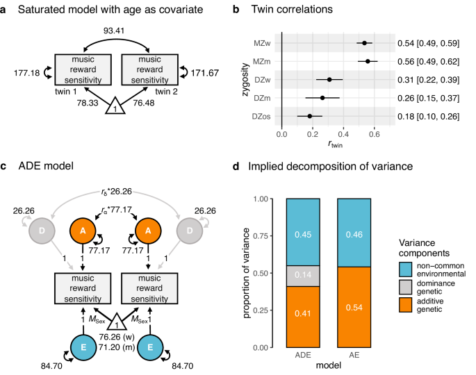
Given that the variance and covariance are measured between twins within families, it is possible to specify a multigroup structural equation model and estimate three out of four variance components. The decision of which parameters to include in the model (e.g., A, C, E, or A, D, E) is purely based on twin covariances, which are extracted from the constrained saturated model phenotypic model (see below), and biological plausibility. If σMZ, MZ > 2*σDZ,DZ, then D is expected to contribute to the phenotypic variance and, therefore, an ADE model is specified. Otherwise, an ACE model is fit to the data.
CTD assumptions
The estimates from the CTD are unbiased under a set of assumptions. First, the CTD assumes equal environments between the twins. In other words, it assumes that similarities between twins caused by the environment are the same for both zygosities. Suppose, instead, MZ twins experience their environment more similarly than DZ twins due to environmental, not genetic, causes. In that case, the estimate for the genetic variance will be upwardly biased (i.e., \(\widehat{{{{\rm{\sigma }}}}_{{{\rm{A}}}}^{2}}\) > σA2). Note that the equal environment assumption is not violated if MZ twins experience their environment more similarly than DZ twins due to genetic differences. The second assumption is that the phenotypes of the parents of the twins are uncorrelated (i.e., random mating, also known as panmixia80). If the covariance between two parental phenotypes, p1 and p2, is different from 0, σP1,P2 \(\ne\) 0, then the shared environmental variance might be upwardly biased (i.e., \(\widehat{{{{\rm{\sigma }}}}_{{{\rm{C}}}}^{2}}\) > σC2). The third assumption is that there are no gene-environment interactions or gene-environment passive correlations. Based on the type of gene-environment interaction or correlation, different sources of bias are expected. If AxC is present, then \(\widehat{{{{\rm{\sigma }}}}_{{{\rm{A}}}}^{2}}\) > σA2 is expected. If AxE is present instead \(\widehat{{{{\rm{\sigma }}}}_{{{\rm{E}}}}^{2}}\) > σE2. If passive rG,E is present, then \(\widehat{{{{\rm{\sigma }}}}_{{{\rm{C}}}}^{2}}\) > σC2 is expected. An additional set of assumptions introduced when estimating parameters via SEM is that means and variances are equal across zygosity group, twin order (i.e., 1 and 2), and sex. Details on the latter set of assumptions are given below. Complex sources of upward or downward biases in CTD-informed models (e.g., heterogeneity) are discussed elsewhere81.
Saturated model
We first fit multigroup SEM models to create a baseline against which to compare the fit of univariate and multivariate models and test for the assumptions of the equality of mean and variances. The models freely estimated all the observed variance and covariances and included the age of the twins as a covariate. For the univariate model, equality of means and variances was tested by sequentially constraining parameters and comparing the Akaike Information Criterion (AIC) and Bayesian Information Criterion (BIC) of the models, where AIC = 2k – 2ln(\(\widehat{{{\rm{L}}}}\)) and BIC = kln(k) – 2ln(\(\widehat{{{\rm{L}}}}\)), with k being the number of parameters estimated in the model and \(\widehat{{{\rm{L}}}}\) the maximised value of the likelihood function. Models with smaller AIC and BIC were deemed a good fit. Additional comparisons are provided by the likelihood-ratio test (LRT), using the lavaan::lavTestLRT() function from the lavaan R package82. All models were specified following lavaan notation and fitted with the lavaan::sem() function.
Univariate variance decomposition
The SEM specification was informed by the CTD, following the pattern of twin pairs correlations extracted from the SEM model selected after model comparison results. Twin pairs correlations were extracted using the most parsimonious constrained saturated model using the lavaan::standardizedSoultion() function. Precisely, we fit a five-group ADE SEM model, where the five groups were formed by either full or incomplete MZ women, MZ men, DZ women, DZ men, and DZ opposite-sex pairs. Means for women and men were estimated freely across sex, but not across zygosities or twin order. We fit the model via the direct symmetric approach by directly estimating the variances, as it can derive asymptotically unbiased parameter estimates and is, therefore, less prone to type I errors83. We then decomposed the variance-covariance matrix T of twin pairs into the T = A + D + E variance covariances, which was predicted as follows:
$${{\bf{T}}}=\left[\begin{array}{cc}{{{\rm{\sigma }}}}_{A}^{2}{+{{\rm{\sigma }}}}_{D}^{2}{+{{\rm{\sigma }}}}_{E}^{2} & {r}_{\alpha } * {{{\rm{\sigma }}}}_{A}^{2}{+{r}_{{{\rm{\delta }}}} * {{\rm{\sigma }}}}_{D}^{2}\\ {{r}_{\alpha } * {{\rm{\sigma }}}}_{A}^{2}{+{r}_{{{\rm{\delta }}}} * {{\rm{\sigma }}}}_{D}^{2} & {{{\rm{\sigma }}}}_{A}^{2}{+{{\rm{\sigma }}}}_{D}^{2}{+{{\rm{\sigma }}}}_{E}^{2}\end{array}\right]$$
(3)
Where rα is the expected additive genetic relationship, and rδ is the expected dominant genetic relationship between pairs (i.e., rα = 1 or 0.5, rδ = 1 or 0.25, for MZ and DZ, respectively). Note that for simplicity, here we exclude the contribution of age to T, which was instead included in the model. To test for the significance of the variance components A and D, we additionally fit two models where D and AD variances were constrained to 0. Significance was inferred by model comparison, as above. We fit the model to the raw sum score of the BMRQ using the lavaan::sem() function. Assuming data within pairs were missing at random, we used the recommended estimator for twin data analysis, the full-information maximum likelihood (FIML; argument estimator = “ML”). We used the following estimator for the heritability:
$${h}_{{twin}}^{2}=\frac{{{{\rm{\sigma }}}}_{A}^{2}}{{{{\rm{\sigma }}}}_{A}^{2}+{{{\rm{\sigma }}}}_{E}^{2}}$$
(4)
Here we note the detail that σA2 + σE2 \(\ne\) σP2, as σP2 = σA2 + σE2 + B2*σAge2. We also note that, since the E component includes residual deviation, σE2 = inter-σE2 + intra-σE2, where inter-σE2 is the inter-individual variance, and intra-σE2 is the intra-individual variance80. Comparisons with standard OpenMX protocols are given in Supplementary Note 7 (note that the small differences in test statistics did not lead to different conclusions). A graphical representation of the full univariate multigroup model can be found in Supplementary Fig. 3.
Cholesky decomposition
We applied a Cholesky decomposition to SMDT, BAS-RR, and BMRQ twin data84. Following the CTD, we specified a multivariate model to estimate path (e.g., λA1 and λE1) and cross-path (e.g., λA12 and λE12) coefficients. The predicted 6 × 6 S symmetric matrix included the within-twin variance covariances on the S1:3,1:3 and S4:6,4:6 elements and the between-twin variance covariances on the S4:6,1:3 and S1:3,4:6 elements. The within-twin variance-covariance matrices were obtained as Aw = XXT or Ew = ZZT, where X and Z are the lower triangular matrices with the path (on the diagonal) and cross-path (on the off-diagonal) coefficients for the additive genetic and environmental components, respectively. The between-twin variance-covariance Ab matrix was obtained similarly but considered the expected additive genetic correlations, rα, between MZ or DZ twins. The sequence of variables was purely chosen to regress out A1 and A2, and E1 and E2, respectively, implied from SMDT and BAS-RR observed scores from the BMRQ. To estimate an adjusted heritability (here, for simplicity, adj-htwin2), we calculated the proportion of variance of the BMRQ covarying with the component A over the total BMRQ variance (minus the variance in BMRQ covarying with age):
$${{adj}-h}_{{twin}}^{2}=\frac{{\lambda }_{A3}^{2}}{({\lambda }_{A3}^{2}+{\lambda }_{E3}^{2})+({\lambda }_{A13}^{2}+{\lambda }_{E13}^{2}+{\lambda }_{A23}^{2}+{\lambda }_{E23}^{2})}$$
(5)
Where the numerical subscripts simply indicate the order of the phenotype in the model (e.g., 3 is the BMRQ). To calculate the amount of additive genetic variance unique and associated with BMRQ beyond SMDT and BAS-RR (σAu:At2; u = unique, t = total), we computed the proportion of genetic variance over the total BMRQ additive genetic variance as follows:
$${{{\rm{\sigma }}}}_{{Au}:{At}}^{2}=\frac{{\lambda }_{A3}^{2}}{({\lambda }_{A3}^{2})+({\lambda }_{A13}^{2}+{\lambda }_{A23}^{2})}$$
(6)
A graphical representation of the full multivariate model can be found in Supplementary Fig. 5. Similar to what was reported above, we fit the models using the lavaan::sem() function (estimator “ML”) but to standardised variables and latent components. We used LRT for the significance of the λ coefficient, where the full model was compared to a model in which any tested λ coefficient was set to be equal to 0.
Distinct factor solution
To estimate the genetic and environmental correlations between facets of music reward, we applied a correlated factor model via a direct symmetric approach83 (referred to as a distinct factor solution). The direct symmetric approach is conceptually similar to a correlated factor solution. In the correlated factor solution, the multivariate phenotypic variance-covariance matrix M is obtained as M = A + E (in the simplest case of an AE model), with A = XRAXT and E = ZREZT, where X and Z are the diagonal matrix of the standard deviation σA and σE and RA is the genetic correlation matrix. Within a direct symmetric approach, instead, a different parametrisation is specified to directly estimate the M 10 × 10 symmetric matrix as M = A + E:
$${{\bf{M}}}=\left[\begin{array}{ccccc}{{{\rm{\sigma }}}}_{A1}^{2}+{{{\rm{\sigma }}}}_{E1}^{2} & {{{\rm{\sigma }}}}_{A1,A2}+{{{\rm{\sigma }}}}_{E1,E2} & \cdots & {r}_{\alpha } * {{{\rm{\sigma }}}}_{A1,A4} & {r}_{\alpha } * {{{\rm{\sigma }}}}_{A1,A5}\\ {{{\rm{\sigma }}}}_{A1,A2}+{{{\rm{\sigma }}}}_{E1,E2} & {{{\rm{\sigma }}}}_{A2}^{2}+{{{\rm{\sigma }}}}_{E2}^{2} & \vdots & {r}_{\alpha } * {{{\rm{\sigma }}}}_{A2,A4} & {r}_{\alpha } * {{{\rm{\sigma }}}}_{A2,A5}\\ \vdots & \vdots & \ddots & \vdots & \vdots \\ {r}_{\alpha } * {{{\rm{\sigma }}}}_{A1,A4} & {r}_{\alpha } * {{{\rm{\sigma }}}}_{A2,A4} & \vdots & {{{\rm{\sigma }}}}_{A4}^{2}+{{{\rm{\sigma }}}}_{E4}^{2} & \vdots {{{\rm{\sigma }}}}_{A4,A5}+{{{\rm{\sigma }}}}_{E4,E5}\\ {r}_{\alpha } * {{{\rm{\sigma }}}}_{A1,A5} & {r}_{\alpha } * {{{\rm{\sigma }}}}_{A2,A5} & \cdots & {{{\rm{\sigma }}}}_{A4,A5}+{{{\rm{\sigma }}}}_{E4,E5} & {{{\rm{\sigma }}}}_{A5}^{2}+{{{\rm{\sigma }}}}_{E5}^{2}\end{array}\right]$$
(7)
Where the M1:5,1:5 and M5:10,5:10 elements include the within-twin variance and between-traits covariances and are constrained to be equal across zygosities, and the M5:10,1:5 and M1:5,5:10 elements include the between-twin additive genetic within- and between-trait covariances and the expected additive genetic relationship rα, which is fixed to either 1 or 0.5 in MZ and DZ groups, respectively. While this approach may return out-of-bound values, the absence of boundaries has been shown to yield asymptotically unbiased parameter estimates and correct type I and type II error rates83. A graphical representation of the full multivariate model can be found in Supplementary Fig. 6. Model syntax was written following lavaan specifications. Model fitting was done via the lavaan: sem() function (estimator “ML”). In sum, the distinct factor solution provides a multivariate model for the decomposition of phenotypic variances and covariances in genetic and environmental components. Comparison of this model with more parsimonious independent pathway models allows us to test for the presence of a shared genetic (or environmental) component shared across facets.
Shared-genetic factor solution
The hybrid-independent genetic pathway model (referred to here as shared-genetic factor solution) is a multivariate approach similar to the correlated factor solution, except with an additional restriction on the genetic covariances between traits (σA,A; hence hybrid or genetic, as environmental covariances are modelled in a distinct factor solution fashion). Consider a 5 × 5 phenotypic variance-covariance matrix P. Under an AE shared-genetic factor solution, P can be written as P = As + Au + E, where As = XsXsT, with Xs being a 5 × 1 vector of the additive genetic path coefficients of a shared additive genetic factor (AC) loading across all phenotypes, and Au is a 5 × 5 diagonal matrix including the residual unique genetic variance for each phenotype, σAu2. The full additive genetic variance-covariance matrix can be then as follows:
$${{{\bf{A}}}}_{{{\bf{t}}}}={{{\bf{X}}}}_{{{\bf{s}}}}{{{\bf{X}}}}_{s}^{T}+{{{\bf{A}}}}_{{{\bf{u}}}}=\left[\begin{array}{ccccc}{{{{\boldsymbol{\lambda }}}}_{A1}^{2}+{{\rm{\sigma }}}}_{{Au}1}^{2} & {{{\boldsymbol{\lambda }}}}_{A1} * {{{\boldsymbol{\lambda }}}}_{A2} & {{{\boldsymbol{\lambda }}}}_{A1} * {{{\boldsymbol{\lambda }}}}_{A3} & {{{\boldsymbol{\lambda }}}}_{A1} * {{{\boldsymbol{\lambda }}}}_{A4} & {{{\boldsymbol{\lambda }}}}_{A1} * {{{\boldsymbol{\lambda }}}}_{A5}\\ {{{\boldsymbol{\lambda }}}}_{A1} * {{{\boldsymbol{\lambda }}}}_{A2} & {{{{\boldsymbol{\lambda }}}}_{A2}^{2}+{{\rm{\sigma }}}}_{{Au}2}^{2} & {{{\boldsymbol{\lambda }}}}_{A2} * {{{\boldsymbol{\lambda }}}}_{A3} & {{{\boldsymbol{\lambda }}}}_{A2} * {{{\boldsymbol{\lambda }}}}_{A4} & {{{\boldsymbol{\lambda }}}}_{A2} * {{{\boldsymbol{\lambda }}}}_{A5}\\ {{{\boldsymbol{\lambda }}}}_{A1} * {{{\boldsymbol{\lambda }}}}_{A3} & {{{\boldsymbol{\lambda }}}}_{A2} * {{{\boldsymbol{\lambda }}}}_{A3} & {{{{\boldsymbol{\lambda }}}}_{A3}^{2}+{{\rm{\sigma }}}}_{{Au}3}^{2} & {{{\boldsymbol{\lambda }}}}_{A3} * {{{\boldsymbol{\lambda }}}}_{A4} & {{{\boldsymbol{\lambda }}}}_{A3} * {{{\boldsymbol{\lambda }}}}_{A5}\\ {{{\boldsymbol{\lambda }}}}_{A1} * {{{\boldsymbol{\lambda }}}}_{A4} & {{{\boldsymbol{\lambda }}}}_{A2} * {{{\boldsymbol{\lambda }}}}_{A4} & {{{\boldsymbol{\lambda }}}}_{A3} * {{{\boldsymbol{\lambda }}}}_{A4} & {{{{\boldsymbol{\lambda }}}}_{41}^{2}+{{\rm{\sigma }}}}_{{Au}4}^{2} & {{{\boldsymbol{\lambda }}}}_{A4} * {{{\boldsymbol{\lambda }}}}_{A5}\\ {{{\boldsymbol{\lambda }}}}_{A1} * {{{\boldsymbol{\lambda }}}}_{A5} & {{{\boldsymbol{\lambda }}}}_{A2} * {{{\boldsymbol{\lambda }}}}_{A5} & {{{\boldsymbol{\lambda }}}}_{A3} * {{{\boldsymbol{\lambda }}}}_{A5} & {{{\boldsymbol{\lambda }}}}_{A4} * {{{\boldsymbol{\lambda }}}}_{A5} & {{{{\boldsymbol{\lambda }}}}_{A5}^{2}+{{\rm{\sigma }}}}_{{Au}5}^{2}\end{array}\right]$$
(8)
The 5 × 5 residual environmental covariance E simply contains the unconstrained residual environmental variances and covariances σE2 and σE,E. The 10 × 10 twin variance-covariance matrix M can then be written as follows:
$${{\bf{M}}}=\left[\begin{array}{cc}{{{\bf{A}}}}_{{{\boldsymbol{t}}}}+{{\bf{E}}} & {{r}_{\alpha } * {{\bf{A}}}}_{{{\boldsymbol{t}}}}\\ {{r}_{\alpha } * {{\bf{A}}}}_{{{\boldsymbol{t}}}} & {{{\bf{A}}}}_{{{\boldsymbol{t}}}}+{{\bf{E}}}\end{array}\right]$$
(9)
Where rα is the expected additive genetic relationship between twins and is fixed to either 1 or 0.5 across MZ and DZ groups, respectively. A graphical representation of the full multivariate model can be found in Supplementary Fig. 9. Model syntax was written in lavaan. Model fitting was done via the lavaan:sem() function. Model comparison between distinct and shared-genetic factor solutions was carried out via the laavan:: lavTestLRT() function. Here, we additionally note that the shared-genetic factor solution is a less parsimonious version of the more commonly used independent pathway model and, therefore, provides a less restrictive and more specific test for a genetic shared factor when compared to the distinct factor solution.
Shared-environmental factor solution
The hybrid-independent environmental pathway model (the shared-environmental factor solution) is a multivariate approach similar to the hybrid-independent genetic pathway model. The 10 × 10 matrix M can then be written as follows:
$${{\bf{M}}}=\left[\begin{array}{cc}{{\bf{A}}}+{{{\bf{E}}}}_{{{\boldsymbol{t}}}} & {r}_{\alpha } * {{\bf{A}}}\\ {r}_{\alpha } * {{\bf{A}}} & {{\bf{A}}}+{{{\bf{E}}}}_{{{\boldsymbol{t}}}}\end{array}\right]$$
(10)
Where Et = Es + Eu, with Es = ZsZsT, Zs being a 5 × 1 vector of the environmental path coefficients of a shared environmental (Es) loading across all phenotypes, and Eu the 5 × 5 diagonal matrix including the residual environmental variance for each phenotype, σEu2.
Six-variate distinct factor solution
We extended the previous five-variate distinct factor solution including either music perceptual abilities or general reward sensitivity. This model allowed us to estimate the genetic and environmental correlations between music perceptual abilities or general reward sensitivity and the five facets of music reward sensitivity. To test for the significance of the differences between genetic or environmental overlap between facets, we compared the full six-variate model with a model in which any of the tested pairwise genetic or environmental covariances were set to be equal. Model comparisons were carried out via the laavan:: lavTestLRT() function.
Structural equation modelling assumptions
SEM-based estimates obtained from the full-information maximum likelihood (FIML) estimator are unbiased under the assumption that observations follow a multivariate normal distribution42. Violation of the assumption of multivariate normality has been found to have little impact on parameter estimates but can have severe consequences for both the χ2 test statistics and the standard error of the estimates for the parameters. An alternative estimator that is less sensitive or robust to violation of multivariate normality is the maximum likelihood with robust standard error and scaled test statistics (MLR). Although this estimator assumes missingness to be completely at random, it has been shown to provide quite reliable estimates of data missing at random85. Relevant comparisons between the two estimators are given in Supplementary Note 1.
Reporting summary
Further information on research design is available in the Nature Portfolio Reporting Summary linked to this article.