Urban and non-urban contributions to the social cost of carbon

CLIMRISK description

CLIMRISK is a recent IAM of the climate and economy which allows projecting the economic impacts and risks of climate change at the global, regional and spatially explicit (0.5° × 0.5°) scales4. It is structured in four main modules: (1) Socioeconomic, which represents exposure in terms of total, urban and non-urban population and GDP; 2) Climate, it is divided in three sections which are a global climate model, a general circulation models emulator to produce spatially explicit temperature and precipitation projections, and a third section that projects UHI intensity in urban areas as a function of population counts; 3) Economic damages, which contains sets of global, regional and grid scale-defined damage functions (DF) to map increases in temperature to losses in GDP. Some of these DFs are time-, path- and scenario-dependent. The different set of damage functions include those based on enumerative and expert judgement28,67,68,69, computable general equilibrium54 and econometric23 approaches; 4) Risk evaluation, it combines the results from the climate and economic damages modules to produce uni- and multi-variate risk indices. Figure 3 shows a stylized description of the core modules of CLIMRISK. The model aggregates results in 13 regions which are described in Table S16, although results are also available at the grid-cell level and for 178 individual countries (Table S17). Note that while higher spatial resolution could be desirable for some analysis, and for potentially more precise estimates, the resolution in CLIMRISK reflects the current constraints in global datasets and computing power available to run the model. The following paragraphs present the improvements in CLIMRISK used in this paper. The reader is referred to the detailed description of the model contained in the Supplementary Information of Estrada and Botzen4.

Fig. 3: Schematic description of CLIMRISK’s model structure.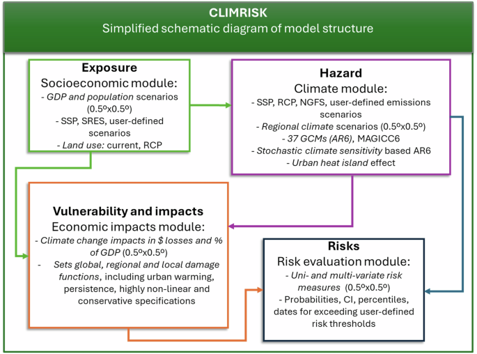

The model is composed of four main modules. The exposure module produces spatially explicit socioeconomic scenarios, including GDP and population from SSP, SRES datasets, as well as from user-defined trajectories. This module also includes RCP land use projections. The hazard module contains a stochastic version of a reduced complexity climate model (MAGICC6) and produces spatially explicit changes in temperature and precipitation by emulating 37 Atmosphere-Ocean General Circulation Models (AOGCMs) of the Coupled Model Intercomparison Project (CMIP6). It also produces estimates of the UHI intensity for urban cells. The vulnerability and impacts module generates projections of the economic impacts of climate change by means of a collection of global, regional and local damage functions, with specifications that range from conservative to highly nonlinear and catastrophic. The estimates produced can include the UHI effect and the persistence of climate change impacts. The risk evaluation module uses the output of the different modules to generate uni- and multivariate dynamic risk indices which can provide a more complete view of climate change risks.

Improvements in CLIMRISK’s climate module

The climate module in CLIMRISK has been updated to reflect some of the recent advances reported in the latest assessment report (AR6) of the IPCC70. CLIMRISK uses a triangular probability distribution to represent the uncertainty of the climate sensitivity parameter in MAGICC671,72, a reduced complexity climate model. The parameters of the triangular distribution have been updated to reflect the very likely range in the AR6. The triangular distribution in the current version of CLIMRISK is specified with 2 °C and 5 °C as the lower and upper limits, respectively, with a most likely value of 3 °C.

CLIMRISK uses the pattern scaling technique73,74,75,76 to generate spatially explicit annual temperature and precipitation scenarios (see ref. 4). Currently, the climate module in CLIMRISK contains a pattern scaling library of 37 Atmosphere-Ocean General Circulation Model (AOGCM) included in the Coupled Model Intercomparison Project (CMIP6). These patterns are produced using ordinary least squares regression as described in the original CLIMRISK paper4 and others75,76,77. Table S18 provides a list of names of the AOGCMs included in the current version of CLIMRISK.

Extension of damage functions in CLIMRISKCountry level and regional damage functions

CLIMRISK includes a variety of global DFs that can be used for the analysis of climate impacts at the regional and local scales, ranging from conservative, highly nonlinear and to catastrophic. For the results shown in the main text of this paper we use a new country and grid-cell level sets of damage functions derived from computable general equilibrium estimates of the economic impacts of climate change54. These damage functions were not available in the previous version of CLIMRISK and were developed for this study. Kompas et al.54 provide country and region estimates of economic damages for different levels of increase in global temperatures (1–4 °C). Using linear regression, a quadratic function of global temperature increase was fitted for each of the 140 countries/regions for which estimates were available, producing an average \({R}^{2}\) of 0.997. These damage functions are denoted in CLIMRISK with the letter K. The regional estimates presented in Kompas et al. (e.g., Rest of western Africa) were used to assign damage functions to countries not explicitly included in their analysis to complete 187 countries. CLIMRISK produces socioeconomic and climate projections at the grid-cell level (0.5° × 0.5°) and to take advantage of this spatially explicit exposure and hazard scenarios, subnational level spatial patterns of damages are produced. The approach used can be described as follows and it is applicable to a variety of damage functions (DF; see ref. 4 for a detailed description):

1. (1)

   The economic impacts for country/region r are calculated using global temperature change, as done in the original non-spatially explicit source54,67:

   $${I}_{t,r}^{{DF}}={\Omega }_{t,r}{Y}_{t,r}=\left[{\beta }_{1,r}{\Delta T}_{t}+{\beta }_{2,r}{\Delta T}_{t}^{2}\right]{Y}_{t,r}$$

   (1)

   Where \({\Omega }_{t,r}\) is the percent of GDP lost due to climate change in country/region r at time t, \({Y}_{t,r}\) is the GDP for country/region r at time t, \({\beta }_{1,r}\) and \({\beta }_{2,r}\) are the linear and quadratic parameters of the damage function DF for country/region r and \({\Delta T}_{t}\) is global temperature change at time t.

2. (2)

   The economic impacts for country/region r are calculated using grid-cell level temperature change and GDP, and country/region damage parameters:

   $${I}_{t,g}^{{DF}}={\Omega }_{t,g}{Y}_{t,g}=\left[{\beta }_{1,r}{\Delta T}_{t,g}+{\beta }_{2,r}{\Delta T}_{t,g}^{2}\right]{Y}_{t,g}$$

   (2)

   $${I}_{t,{r}^{*}}^{{DF}}=\sum\limits_{g}{I}_{t,g}^{{DF}}$$

   (3)

   Where g is the set of geographical coordinates (latitude, longitude) that correspond to each grid-cell in country/region r. \({I}_{t,{r}^{*}}^{{DF}}\) is the sum of economic losses in all grid cells in country/region r.

3. (3)

   The subnational spatial patterns of impacts based on grid-cell exposure and hazard are constructed and damages are rescaled to match \({I}_{t,r}^{{DF}}\) at the country/regional level:

$${{SP}}_{t,g}^{{DF}}={I}_{t,g}^{{DF}}/{I}_{t,{r}^{*}}^{{DF}}$$

(4)

$${I}_{t,g}^{{{DF}}^{*}}={{SP}}_{t,g}^{{DF}}\cdot {I}_{t,r}^{{DF}}$$

(5)

Where \({I}_{t,g}^{{{DF}}^{*}}\) are the spatially explicit projected damages consistent with the original, country/region aggregated estimate \({I}_{t,r}^{{DF}}\). In the case of the Kompas damage functions, the corrected estimates are referred to as \({I}_{t,g}^{{K}^{*}}\).

Grid-cell level damage functions

Grid-cell level damage functions were derived from Kompas et al. taking advantage of the existing relationship between their country level damage estimates and the reported national Human Development Index56 (HDI; Fig. 4). Previously, downscaling of damages has been done based on per capita income78. Here we chose HDI because it is a comprehensive indicator that accounts for income, education and health and it has been shown to outperform several indices of social vulnerability to climate change79,80,81. As expected, high/low scores in the HDI are associated to lower/higher vulnerability to climate change (Fig. 4) This relationship was estimated using the following linear regression:

$${{{\mathrm{ln}}}}\, {D}_{r}^{K}={b}_{1}{{HDI}}_{r}+{b}_{2}{{HDI}}_{i}^{2}+\sum\limits_{i=1}^{4}{\gamma }_{i}{l}_{i}+{\varepsilon }_{i}$$

(6)

Where \({D}_{r}^{K}\) are the economic damages reported in Kompas et al.54 for the country r, \({{HDI}}_{r}\) are the corresponding HDI scores, and \({l}_{i}\) are dummy variables for the different levels of warming the estimates in Kompas et al. were reported (1–4 °C). This regression produces an \({R}^{2}\) of 0.62. The out-of-sample forecast performance was evaluated by retaining 119 observations, which led to a Theil inequality coefficient of 0.28, with a covariance proportion of 0.993, and bias and variance proportions of less than 0.01. Using spatially explicit HDI estimates, \({D}_{r}^{K}\) was projected onto a 0.5° × 0.5° grid and local scale damage functions (60,000+) were constructed following the linear regression approach described before.

Fig. 4: Scatterplot of \({D}_{r}^{K}\) and. \(HD{I}_{r}\) with a quadratic regression fit.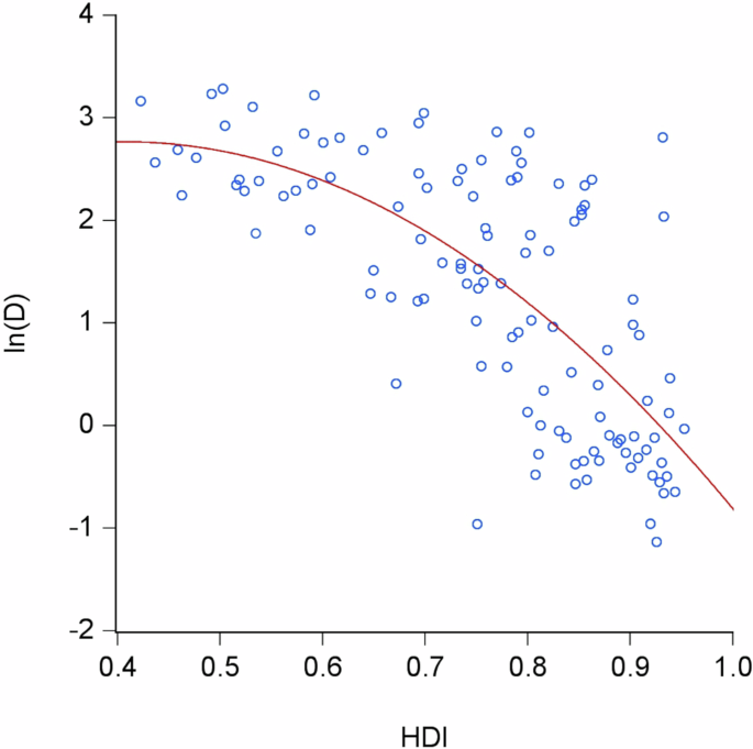

Blue circles represent the relationship between projected climate change economic impacts (\({{{{\boldsymbol{D}}}}}_{{{{\boldsymbol{r}}}}}^{{{{\boldsymbol{K}}}}}\)) and the Human Development Index (\({{{{\boldsymbol{HDI}}}}}_{{{{\boldsymbol{r}}}}}\)) across 140 countries. The red line shows the fitted quadratic regression curve.

With these grid cell estimates the Eq. (2) in step 2) was replaced by:

$${I}_{t,g}^{{DF}}={\Omega }_{t,g}{Y}_{t,g}=\left[{\beta }_{1,g}{\Delta T}_{t,g}+{\beta }_{2,g}{\Delta T}_{t,g}^{2}\right]{Y}_{t,g}$$

(7)

The regularization described in step 3) was applied to ensure consistency with the original estimates in Kompas et al.54, producing the \({I}_{t,g}^{K}\) estimates. As discussed in the following sections, CLIMRISK identifies grid cells that contain urban areas and the local UHI warming can be incorporated into the urban area temperature projection. For these areas the corresponding K grid cell damage function adjusted using its HDI value is used to project urban damages. The KU estimates combine the \({I}_{t,g}^{K}\) estimates with local damage functions in urban areas that include UHI warming (see below for a description).

The Supplementary Information includes a sensitivity analysis based on updated versions of CLIMRISK’s R and RU damage functions. The global damage function that was selected for the update is the DICE2016R28, which is still widely used. Note that other global/regional damage functions can be chosen, such as those that focus on catastrophic climate change68,82. The R and K sets of damage functions provide contrasting views about the seriousness of climate change impacts to the global economy, with the DICE2016R commonly considered as conservative.

To produce these updated versions of the R damage functions, the following steps are conducted:

1. a.

   To produce the grid-cell level estimates consistent with the regional RICE2010 damages, steps 1) to 3) described in the previous section are applied to produce \({I}_{t,g}^{{R}^{*}}\).

2. b.

   The total global damage for time t is calculated summing over all g coordinates in all regions, \({I}_{t}^{{R}^{*}}={\sum}_{g}{I}_{t,g}^{{R}^{*}}\).

   The grid-corrected, regional consistent \({I}_{t,g}^{{R}^{*}}\) are used to construct the spatial patterns (downscaling patterns) for the RICE2010.

   $${{SP}}_{t,g}^{{R}^{*}}={I}_{t,g}^{{R}^{*}}/{I}_{t}^{{R}^{*}}$$

   (8)

3. c.

   The global damages are calculated using the target global damage function driven by global temperature change \({I}_{t}^{{target}}=\Phi \left({\Delta T}_{t}\right){Y}_{t}\), where \({Y}_{t}\) is global GDP at time t.

4. d.

   The estimates of the target damage function \({I}_{t}^{{target}}\) downscaled using the RICE2010 grid-cell/regional spatial patterns are obtained as:

$${I}_{t,g}^{{target}}={{SP}}_{t,g}^{{R}^{*}}\cdot {I}_{t}^{{target}}$$

(9)

In addition, features in CLIMRISK such as the inclusion of the UHI effect can be incorporated, given rise to modified versions of the RU DFs, as described in ref. 4 and ref. 50. For simplicity of notation, we will still refer to the updated versions these damage functions as R and RU.

Definition of urban areas

In the previous version of CLIMRISK4, urban areas were declared in grid cells with population counts larger than 1 million inhabitants. This calibration was found to be very conservative as it led to underestimating the global urban population (about 40%) and GDP (about 50%). In the current version of the model, two approaches are used. The first approach consists of replicating the urban population projections available for each of the SSP trajectories83 by optimizing for each region the population threshold parameter that is used in CLIMRISK to determine urban grid cells. The optimization procedure consists in minimizing the sum of squared residuals between the original and fitted regional urbanization projections by varying the urban threshold parameter over a wide range of values (1000 and 3.5 million inhabitants in steps of 10,000 inhabitants) per grid cell in each region. This was done for the period 2010–2100 in 10-year time steps. Fig. 5 compares the SSP5 urbanization shares projections in ref. 83. with those of CLIMRISK for each of the 13 regions used in this paper. At the global level under the SSP5 scenario, the urban population share starts at 50% in 2010 and reaches about 90% in 2100. The urban GDP that corresponds to the identified urban cells corresponds to 70% in 2010 and about 90% in 2100. As mentioned below, these figures are broadly consistent with estimates of global urban population and GDP shares. The proportion of urban population varies substantially among the different SSP trajectories, with the lowest levels of urbanization occurring under the SSP3, reaching about 60% at the end of the century (Fig. S3). The projections of urban population and GDP shares for different SSP scenarios are shown in Fig. S4.

Fig. 5: SSP5 projections of urban population shares for 13 regions in CLIMRISK.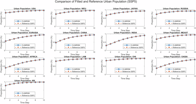

The reference SSP5 urban population shares projections are shown in slashed red lines and the fitted CLIMRISK projections are shown in blue continuous lines.

The Supplementary Information presents a sensitivity analysis of the main results in the main text using a second approach for determining urban populations shares (Fig. S2, Tables S14 and S15). This second approach is based on selecting a global population count threshold which is calibrated to align with observed estimates of the percentages of global urban population and GDP. These estimates are uncertain, but urban population is estimated to represent between 56% and 85% of the total global population39,84. The population count threshold per grid cell to declare a urban area was chosen to be 250,000 inhabitants, which leads to population counts that represent about 62% of global population and about 78% of global GDP in 2010, which is aligned to estimates in the literature36,38,85. In the grid cells that are identified as containing urban areas 75% of the population and 95% of GDP are assumed to be urban. These quantities are used to calculate the UHI and the urban GDP that is subject for the urban damage function that is explained next.

Projecting the UHI intensity in CLIMRISK

The intensity of the canopy UHI has been estimated in the literature by observation-based methods, physical climate models and by empirical-statistical relationships. The first two are mostly available for a restricted number of cities due to the data quality and availability requirements, as well as to large computational costs in the case of physical models. Moreover, damage functions are calibrated for climatological (i.e., long-term) values of changes in global and/or local temperature change. Such estimates are rarely found in the literature using physical climate models or observational estimates. Empirical-statistical methods take advantage of correlations between UHI intensity and variables representing changes in local conditions, such as population41,86,87, land cover, and elevation88. CLIMRISK projects the intensity of the UHI based population counts per grid cell using the following functional form87,89,90,91

$${UHI}=a\times {{Pop}}^{b}$$

(10)

where \(a=0.00174\) and \(b=0.45\) and \({Pop}\) is the population count as in ref. 4,92. The projected values of UHI intensity in CLIMRISK are broadly similar to those one of the few global studies of UHI using a global physical climate model4,93. For the SSP5, the average city has a UHI intensity of 0.83 °C, while for grid cells with more than 1 million inhabitants the average UHI intensity is 1.17 °C, which agrees with estimates in the literature94.

The UHI effect and the urban damage functions in CLIMRISK

Consider a Nordhaus-type damage function \(D\left(T\right)=\alpha {T}^{2}\), where \(D\) are the projected losses in GDP (%) which are a function of temperature change \(T\). Including local temperature change caused by the UHI effect in urban areas results in:

$$D\left(T\right)= {D}_{R}\left({T}_{R}\right)+{D}_{U}\left({T}_{U}\right)={D}_{R}\left({T}_{{GHG}}\right)+{D}_{U}\left({T}_{{GHG}}+{T}_{{UHI}}\right)\\= {\alpha }_{R}{T}_{{GHG}}^{2}+{\alpha }_{U}{\left({T}_{{GHG}}+{T}_{{UHI}}\right)}^{2}=\alpha {T}_{{GHG}}^{2}+2{\alpha }_{U}{T}_{{GHG}}{T}_{{UHI}}+{\alpha }_{U}{T}_{{UHI}}^{2}\\= D\left({T}_{{GHG}}\right)+2{\alpha }_{U}{T}_{{GHG}}{T}_{{UHI}}+{\alpha }_{U}{T}_{{UHI}}^{2}$$

(11)

Where \({D}_{R}\) and \({D}_{U}\) represent losses in rural and urban areas, \({T}_{{GHG}}\) is the change in temperature due to global warming (i.e., anthropogenic forcing), and \({T}_{{UHI}}\) is local warming in urban areas due to the UHI. In words, total damage equals rural damage plus urban damage. Urban temperature change equals rural warming plus urban warming. If the damage is a power (=2) function in temperature, total damage equals total damage of greenhouse warming plus urban damage of urban warming plus the interaction of urban and greenhouse warming. Ignoring the urban heat island effect, \({T}_{{UHI}}=0\), as is done in other integrated assessment models downward biases economic losses4,50.

Modelling of a CO2 pulse in global temperature

The estimation of the SCC requires introducing the effects on temperatures from a pulse in CO2. In this version of CLIMRISK we adopt the approximation proposed by Ricke and Caldeira95 (which is physically sound and easy to implement in IAMs. Following the authors, the effect of a pulse of 1GtC on global temperatures can be approximated using three-exponential functions:

$$\Delta {T}_{t}=-\left({a}_{1}+{a}_{2}+{a}_{3}\right)+{a}_{1}{e}^{-\frac{\left(t-{t}_{0}\right)}{{\tau }_{1}}}+{a}_{2}{e}^{-\frac{\left(t-{t}_{0}\right)}{{\tau }_{2}}}+{a}_{3}{e}^{-\frac{\left(t-{t}_{0}\right)}{{\tau }_{3}}}$$

(12)

Where \({a}_{1}=-\!2.308\), \({a}_{2}=0.743\), \({a}_{3}=-\!0.191\), \({\tau }_{1}=2.241\), \({\tau }_{2}=35.750\), \({\tau }_{3}=97.180\) (see ref. 95). The units of \(\Delta {T}_{t}\) are mK/GtC. The year of the pulse \(({t}_{0})\) is chosen to be 2010.

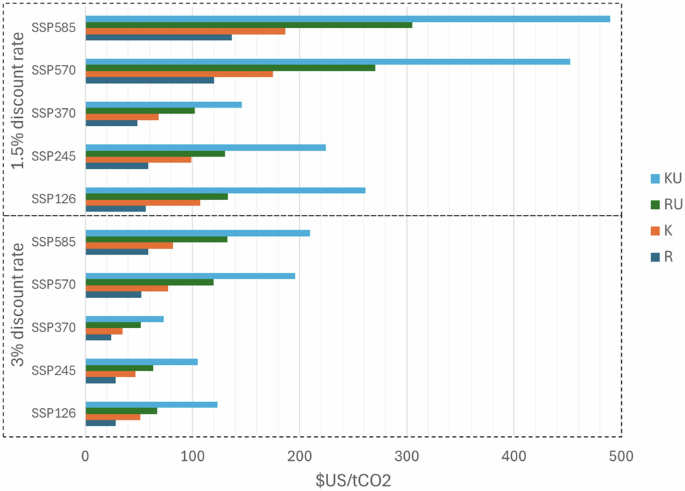
SCC calculation

The SCC values presented in the main text were calculated using a 1.5% discount rate and a sensitivity analysis based on a 3% discount rate are included in the main text (Fig. 1) and in the Supplementary Information (Tables S6–S10). The selection of discount rates is based on recent survey96 which places the social discount rate between 1% and 3% and the 1.7% discount rate suggested in the Circular A-4 of the Office of Management and Budget97 which provides guidance for federal agencies on the development of regulatory analysis. The terminal year for calculating the SCC is 2100 as is common practice in integrated assessment modelling due to the availability of socioeconomic and climate projections under the SSP scenarios.

Decomposing the SCC into urban and non-urban contributions

We use CLIMRISK’s explicit spatial resolution and special modelling of urban areas to calculate SCC values and to decompose these figures into dominantly urban and non-urban (mixed and rural) contributions. Moreover, exploiting the set of damage functions included in CLIMRISK, it is possible to disaggregate the influences of urban exposure and effects from UHI and urban sensitivity, including their interaction with exposure.

In what follows we explain the procedure to compute urban and non-urban SCC for the K and KU DFs. Note that the same decomposition applies to the R and RU type of DFs. First, the total SCC value \(({SC}{C}^{{KU}})\) is the sum of the non-urban \({SC}{C}^{{nu},K}\) and urban \({SC}{C}^{u,{KU}}\) values. In the \({SC}{C}^{{xx},{YY}}\) terms, xx refers to the type of grid cell with nu and u denoting non-urban and urban, respectively, and YY refers to the type of DF used K (without urban effects) and KU (with urban effects). As such, \({SC}{C}^{{nu},K}\) represents the SCC from non-urban grid cells using the K DF (i.e., no urban effects are included), and \({SC}{C}^{u,{KU}}\) is the SCC from urban cells when the UHI effect is considered (KU DF). This can be expressed by the following equation:

$${SC}{C}^{{KU}}={SC}{C}^{{nu},K}+{SC}{C}^{u,{KU}}$$

(13)

the urban SCC estimates (\({SC}{C}^{u,{KU}}\)) can be further decomposed in: 1) the contribution of exposure and; 2) the combined effects of hazard (including UHI), the differences in sensitivity of the urban area to changes in climate and the interaction of these factors and exposure. The contribution of increased exposure in urban areas is obtained by calculating the SCC in urban areas without considering damages from urban effects (i.e., using the K DF) and is denoted by \({SC}{C}^{u,K}\). The contribution of the urban effects (including the UHI) plus interactions is \({SC}{C}^{u,K{U}^{-}}=[{SC}{C}^{u,{KU}}-{SC}{C}^{u,K}]\), the difference between the SCC value from urban grids considering the damages from urban effects \({SC}{C}^{u,{KU}}\) and \({SC}{C}^{u,K}\). \({SC}{C}^{u,K{U}^{-}}\) is referred to as UHI+int in Table 2. The complete decomposition is given by:

$${SC}{C}^{t,{KU}}={SC}{C}^{{nu},K}+{SC}{C}^{u,{KU}}={SC}{C}^{{nu},K}+{SC}{C}^{u,K}+{SC}{C}^{u,K{U}^{-}}$$

(14)

This decomposition allows us to compare the role of exposure concentration in cities under global climate change with the contribution of local climate change and urban sensitivity, within the context of global climate change (i.e., allowing for their interactions and the effect of exposure concentration). Note that both \({SC}{C}^{{nu},K}\) and \({SC}{C}^{u,K}\) share the same damage function (sensitivity) and that, in both cases, damages are driven by global climate change alone. Differences in damages are solely due to dissimilarities in exposure and hazard levels from global warming due to location.

Finally, we define \({SC}{C}^{d,K}={SC}{C}^{u,K}-{SC}{C}^{{nu},K}\) as the change in SCC produced by an additional tonne of CO2 between urban and non-urban context derived only from differences in exposure and global climate change. \({SC}{C}^{d,K}\) is referred to as Inc-Exposure in Table 2. In contrast, \({SC}{C}^{u,K{U}^{-}}\) in Eq. (14) represents the increase in SCC due to urban characteristics including local climate change (UHI), vulnerability, and the interactions between local and global climate change, as well as exposure. This information can be of use for decision-makers at the city level to better understand and address local and global climate change impacts, vulnerability, and adaptation. The proposed separation can be readily applied to the RU functions.