
Performance comparison of the employed model
The performance of the hybrid machine learning models—GOA-XGB, SHO-XGB, and LSA-XGB for predicting the shear strength of UHPC beams is presented in Tables 3 and 4. This analysis provides both the training and testing phases of models. It gives an overall assessment of the prediction performance, error, and reliability of each model, which are paramount in civil engineering applications. Starting with the R2 score, which measures how well each model explains the variance in the data, all models exhibit exceptionally high R2 values during the training phase: GOA-XGB gets 0.9941, SHO-XGB gets 0.9943, and LSA-XGB gets a slightly lower score of 0.9912. These values indicate that each model accounts for about 99% of the variability of the shear strength data and thus provides a good fit to the training dataset.
Table 3 Performance analysis during the training phase.Table 4 Performance analysis during the testing phase.
Nonetheless, the 0.001 difference in R2 scores of the LSA-XGB may imply that it is less likely to over-fit compared to the training phase, since tested again during the testing phase. In the testing phase, coefficients of determination, R2 scores, decrease a bit, which is normal because models work with unknown data. Despite this decrease, the R2 values remain high: The R2 score of GOA-XGB is 0.9570, SHO-XGB is 0.9594, and the best R2 score is achieved by LSA-XGB with 0.9802. This high accuracy can be attributed to the LSA feature to efficiently explore the hyperparameter space of the XGB model without exaggerating the training data54. This shows that LSA-XGB outperforms the other models in terms of generalization, especially because the model complexity is well-balanced with the data fitting capability. The result showed enhanced prediction capacity compared to previous existing research works14. The testing phase results indicate that LSA-XGB can be the most suitable model for practical use when it is crucial to predict the results of new data. Other evaluation criteria that show the accuracy of each model are the RMSE and MAE. In the training phase, the RMSE values are very low for GOA-XGB at 0.0104, SHO-XGB at 0.0102, and LSA-XGB at 0.0127. This pattern is consistent with the MAE values: The results show that GOA-XGB has the lowest error at 0.0069, followed by SHO-XGB at 0.0071, while LSA-XGB has a slightly higher error at 0.0089. These low error values are able to substantiate the fact that the models yield near-correct predictions in the training phase. In the testing phase, RMSE and MAE values increase slightly, which is the expected drop in performance on new data. GOA-XGB has an RMSE of 0.0318 and an MAE of 0.0210; SHO-XGB has an RMSE of 0.0309 and an MAE of 0.0212; and LSA-XGB has slightly better results with an RMSE of 0.0306 and an MAE of 0.0208. The results of the testing phase indicate that LSA-XGB has a more appropriate level of generalization because the corresponding RMSE and MAE values are lower.
Further supporting the models’ credibility and stability are the A20 index, W(I), VAF, and U95 measures. The a20 index, which quantifies the proportion of predictions that are within a 20% range, is very small in the training set at about 0.0008 and slightly higher in testing. Such a low a20 index shows that the models’ predictions are very near reality and are quite precise. The WI values, which are near 1.0 for both training (0.9985) and testing (0.9886) sets, showed that the models have good conformity with the observed values and that the models are consistent. VAF values are above 95% for both phases, indicating that the models are good at reproducing almost all the data variability, with training VAFs peaking at 99.4%. The low U95 values in both phases suggest that there is little variability in the prediction, which is beneficial for the application of the models. Therefore, the high R2 values, low RMSE and MAE, high WI and VAF, and low U95 indicate that GOA-XGB, SHO-XGB, and LSA-XGB are very efficient in predicting the shear strength of UHPC beams. Even in the training phase, GOA-XGB and SHO-XGB have a high accuracy, but in the testing phase, LSA-XGB has a higher R2 score, fewer errors, and thus is the ideal model for use in practice. These findings demonstrate the effectiveness of hybrid machine learning models in improving structural prediction reliability in civil engineering, offering dependable tools to enhance UHPC design, material efficiency, and safety.
Further, Figs. 4 and 5 illustrate scatter charts of the measured shear strength (Vu, test) as well as the shear strength predicted by the ML models (Vu, pred). In these plots, the horizontal axis represents the test values, and the vertical pace shows the Vu and pred values. The greater the accordance of the dots with the black diagonal line that corresponds to y = x, the better the correspondence of the ML model to the distribution of the effect of input factors on the predicted shear strength. Notably, when comparing Figs. 4 and 5, most predicted points from all ML models for the test dataset closely align with the y = x line, as all models were optimized on the training dataset using different techniques. This means that for all the ML models generated, we can confirm that, indeed, they fit the data. In Fig. 4, which presents the results for the training datasets, the predicted strength values are closely aligned with the actual strength values across all three models. This strong correlation is visually apparent through the tight clustering of data points around the best-fit line, indicating a high level of predictive accuracy. For the GOA-XGB model, represented by red data points, most predicted values closely follow the actual strength values, with minimal deviation. Only a small number of points stray from the best-fit line, suggesting that the model is well-tuned to the training data.
Fig. 4
Actual vs. Predicted plot in training datasets.
Fig. 5
Actual vs. Predicted plot in testing datasets.
The SHO-XGB model, shown in yellow, also displays a strong fit, although some deviations are observed at higher strength values. Despite these minor variances, the majority of data points remain close to the best-fit line, indicating that the SHO-XGB model performs reliably on the training data. Meanwhile, the LSA-XGB model, represented by blue points, demonstrates the highest level of accuracy among the three models. The predicted values almost perfectly follow the actual strength values, with very few points deviating from the best-fit line, showing that this model has been finely tuned to the characteristics of the training data. In Fig. 5, which illustrates the performance of these models on the testing datasets, the overall trends remain consistent. However, there is a slight increase in variability when compared to the training data. The GOA-XGB model, again represented by red points, shows a strong correlation between predicted and actual strength values. However, a few more deviations are noticeable in the higher strength ranges, indicating a slightly reduced accuracy when applied to unseen data. Nevertheless, the majority of points still align closely with the best-fit line, demonstrating the model’s strong predictive capability even on the testing set.
For the SHO-XGB model, displayed in yellow, the predicted values continue to follow the actual strength values closely, though the variance in mid-range strength values is more pronounced compared to the training set. This suggests that while the model generalizes well to unseen data, it may show a slight decline in performance at certain strength ranges. However, it still maintains a reasonably strong overall correlation, as most data points cluster near the best-fit line. The LSA-XGB model, represented by blue dots, again shows the best performance with the least error between the predicted and actual values, including the testing set. The majority of the predicted values are still quite accurate in terms of the actual strength values, and the points are clustered around the regression line. This agreement across both the training and testing sets shows that the LSA-XGB model has excellent out-of-sample prediction ability and is ideal for usage in both the training and testing datasets. In general, the comparison between Figs. 4 and 5 shows that the XGB models are quite reliable. Although the accuracy is slightly lower when the model is applied to the test data, the models, especially LSA-XGB, remain quite effective. The figures taken all together underscore the models’ capacity for identifying the structure of the data in the training set and then reproducing that performance in the testing set – a key factor for successful use in practical applications. The LSA-XGB model, for instance, demonstrates a high level of stability in the obtained accuracy across both datasets, thus being the most suitable model for strength values forecasting in this analysis.
Model evaluation and validation techniques
Figure 6 shows the RMSE convergence of the three models used in this study, namely GOA-XGB, SHO-XGB, and LSA-XGB. The first axis on the graph is the number of iterations, while the second one is the RMSE values. The graph gives information on how each model takes to converge and obtain the minimum error that it can perform during training. The GOA-XGB model, depicted by the red line, has the fastest rate of convergence to an RMSE of about 74 in a few iterations. The sharp decrease in RMSE indicates that the model quickly learns and adjusts its predictions during the initial stages of training, finding the optimal solution efficiently. The SHO-XGB model is shown in the blue line, and it is observed that it has a higher RMSE at the beginning of the iterations than the other models, but it gradually reduces after some iterations. However, in the final analysis, the RMSE is approximately 76, which shows that the model provides a slightly less precise solution than the GOA-XGB and LSA-XGB. The LSA-XGB model, shown in green, also exhibits a similar convergence trend to the GOA-XGB model but with a slightly higher initial RMSE. Following a sharp fall in RMSE, the LSA-XGB model attains the minimum error of about 73, suggesting that it is the most efficient of the three models in terms of this metric.
Fig. 6
Convergence curve of all employed model.
The convergence differences between GOA-XGB, SHO-XGB, and LSA-XGB are because the former two models have a more efficient exploration–exploitation strategy. The GOA-XGB quickly decreased the RMSE by presetting on good solutions at the beginning of the process, which reduces the convergence time, albeit slightly reducing the final solution’s accuracy52,60. SHO-XGB is a very slow learning algorithm, which tries to avoid RMSE minimum’s pitfalls of getting caught up in local minima and thus has a slightly higher RMSE53,61. LSA-XGB can achieve both the highest exploration and the highest refinement, the fastest convergence and the lowest RMSE, thus being the most accurate of the three54.
In summary, Fig. 6 shows that all three models can converge, but the LSA-XGB model is the most efficient in terms of RMSE, followed by the GOA-XGB model. The SHO-XGB model, although still effective, exhibits a higher error value, indicating that there is potential for further improvement. From the above convergence behaviour comparison, it is now clear that different models have unique efficiency and accuracy while training.
Additional statistical analysis was carried out to confirm the robustness and generalizability of the used models. The bootstrap residual resampling result of the LSA-XGB model, as shown in Fig. 7 indicates a good fit between the predicted and true value of shear strength with a small 95 percent prediction interval. This suggests that the model is quite stable and substrata by biased with resampling. The histogram of the residuals in Fig. 8 shows that they are normally distributed around zero, indicating that the errors are random and that the model is not too seriously overfitted.
Fig. 7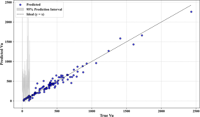
Bootstrap residual resampling.
Fig. 8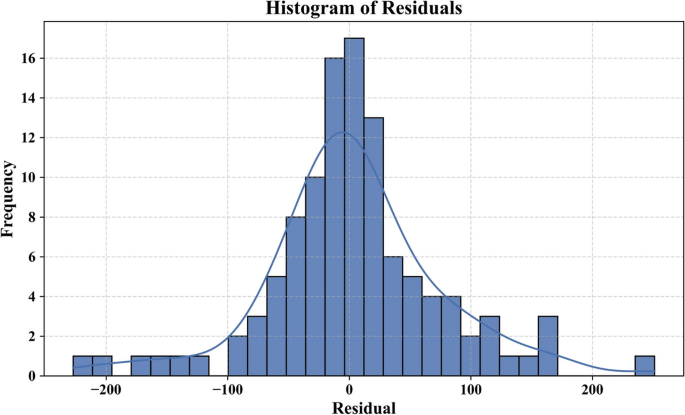
Model residual error of the best model.
Lastly, Fig. 9 indicates the tenfold cross-validation of GOA-XGB, SHO-XGB, and LSA-XGB. Both LSA-XGB and the other methods have high values of R2 in all folds, showing that they have good generalization performance. These tests support the reliability, accuracy, and resilience of the intended models to unexpected data division and random resampling.
Fig. 9
Cross validation of employed models in tenfold.
Data visualization
Figure 10 presents the Regression Error Characteristic (REC) curves for the GOA-XGB, SHO-XGB, and LSA-XGB models on both training and testing datasets. These curves provide a visual comparison of the accuracy of each model as a function of normalized absolute deviation. The x-axis shows the normalized absolute deviation, while the y-axis represents accuracy. The Area Under the Curve (AUC) is included as a measure of the overall performance for each model. In Fig. 10a, which depicts the performance on the training dataset, the LSA-XGB model (green curve) demonstrates superior performance with the highest AUC of 0.905, indicating that this model has the best accuracy for predicting training data. The SHO-XGB model (blue curve) follows with an AUC of 0.885, showing good accuracy but falling slightly short of LSA-XGB. The GOA-XGB model (red curve) has an AUC of 0.868, making it the least accurate of the three on the training set but still within acceptable performance limits.
Fig. 10
Regression Error Characteristics (REC) Curve (a) Training set (b) Testing Set.
In Fig. 10b, the REC curves for the testing dataset reveal a similar trend, although the AUC values are slightly lower across all models. The LSA-XGB model remains the most accurate with an AUC of 0.819, followed closely by the SHO-XGB model with an AUC of 0.812. The GOA-XGB model, with an AUC of 0.815, also performs well, though all models show a small decrease in accuracy when applied to the testing data compared to the training data. The AUC differences stem from the fact that each model uses a different optimization approach. LSA-XGB outperforms all other models in terms of AUC because it finds a golden path in exploration and focused refinement, whereby it avoids many errors and can learn well from testing data. SHO-XGB has a wider scope but is not as precise when it comes to tuning, hence a slightly lower accuracy. GOA-XGB has a high convergence rate, which is good, but at the cost of the final accuracy, resulting in the lowest AUC. Therefore, LSA-XGB is the most reliable for accurate predictions with minimal deviation due to the balanced approach. The REC curves clearly illustrate the comparative effectiveness of each model in reducing prediction errors. A higher AUC indicates better overall performance, with the LSA-XGB model consistently demonstrating the best results on both training and testing datasets. These results provide strong evidence that the LSA-XGB model is the most reliable for making accurate predictions with minimal deviation.
Model explainability
Explaining how a machine learning model arrives at its predictions is essential for interpreting results, especially in complex models. SHAP provides a robust framework for assessing the contribution of each feature to the model’s output. Figures 8, 9, and 10 collectively offer a deep dive into model explainability by utilizing SHAP values to illustrate the impact of individual features on the predictions. Figure 8 displays the Mean Absolute SHAP Value Plot, which ranks the features based on their average SHAP values, showing their overall importance in influencing the model’s predictions. Here, the feature Ac stands out with the highest mean SHAP value of 193.27, indicating that it has the strongest effect on the model’s decisions. Other features like m (109.60) and pf (42.66) also play significant roles, but with a lesser impact compared to Ac. Features at the lower end of the scale, such as lf (2.61) and bf2 (1.94), have minimal influence on the model’s predictions. This ranking helps to identify the key drivers behind the model’s outputs and gives insight into which features are most influential.
Figure 11 goes further by presenting a SHAP Summary Plot, which visualizes how each feature value affects the model’s predictions. The x-axis shows the SHAP values, and the color gradient (from blue to red) represents the range of feature values, where blue indicates lower values and red represents higher ones. For the feature Ac, a wide distribution of SHAP values is observed, showing both positive and negative impacts on the predictions. Higher values of Ac (red) generally push the predictions upwards, while lower values (blue) reduce the predictions. A similar pattern is observed for features like m and pf, where higher feature values are associated with increased SHAP values, indicating a positive influence on the predictions. This plot allows for a better understanding of not only which features are important but also how changes in feature values influence the model’s predictions.
Fig. 11
Mean absolute SHAP value plot.
Figure 12 takes a closer look at individual relationships between feature values and their SHAP values through a series of SHAP Scatter Plots. These scatter plots illustrate how each feature’s value directly affects its contribution to the model’s predictions. For instance, the feature Ac shows a strong positive correlation between higher values and increased SHAP values, suggesting that higher Ac values significantly boost the model’s predicted output. In contrast, features like pf demonstrate a negative correlation, where higher feature values lead to lower SHAP values and, consequently, lower predictions. Certain features, such as bf2 and df, exhibit smaller ranges of SHAP value changes, indicating that they play a less critical role in the overall prediction process. These plots provide detailed insights into the behavior of each feature and how its values influence the model’s output. In conclusion, Figs. 11, 12, and 13 provide a thorough analysis of model explainability using SHAP values. Figure 11 identifies the most important features, while Fig. 12 illustrates how variations in feature values impact predictions. Finally, Fig. 13 offers a closer look at the specific relationships between feature values and their contributions to the model’s output. Together, these figures provide a clear understanding of the model’s decision-making process and highlight which features are driving the predictions.
Fig. 12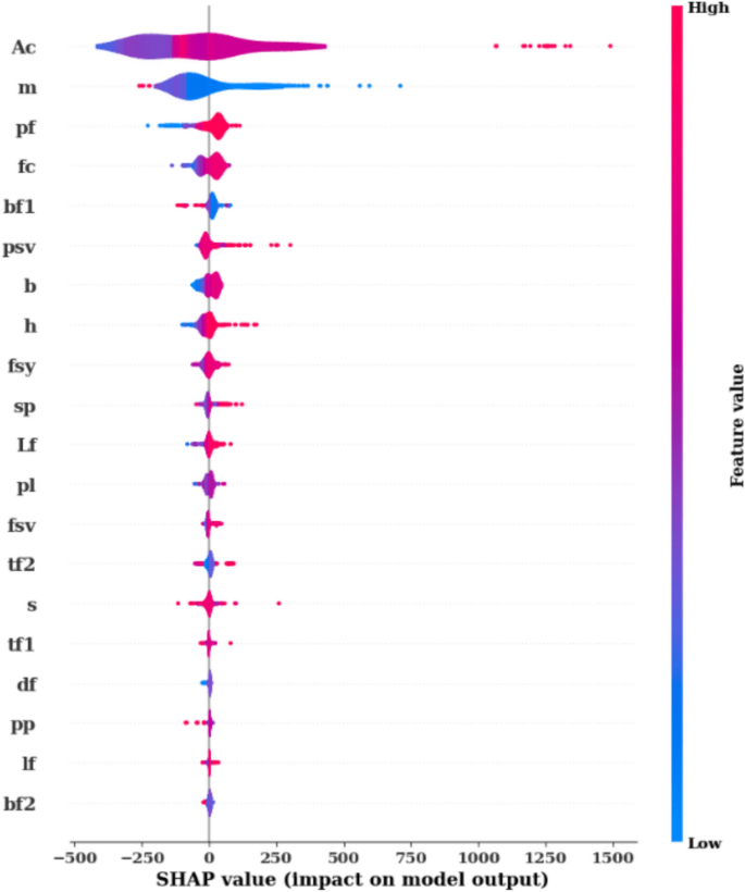 Fig. 13
Model explainability using SHAP values.
Besides the insights of the SHAP-based model, the Sobol global sensitivity analysis was also performed to measure the impact of input features on the model output. The total-order Sobol index indicates that Ac has a significant effect on the predicted shear strength (ST > 0.8), as shown in Fig. 14, and this confirms its dominant influence. m has a very small yet significant contribution, whereas the other features all have a very negligible influence. This homology of SHAP with Sobol outcomes increases the trust in the interpretation of feature importance and confirms that the decision-making process of the model is solid.
Fig. 14
Sobol senstitivity analysis.
Comparison with existing empirical equations
Various existing codes are present to determine beams’ shear capacity, developed based on experiments, theories, and assumptions. However, the shear mechanism is complex as numerous parameters are involved. All of these parameters are hard to include in a single equation. The standard parameters for the shear capacity are section size, axial compressive strength, axial tensile strength, transverse reinforcement, longitudinal reinforcement, fiber factor, etc. Since the existing codes are based on some assumptions, getting precise results is difficult, making it necessary to modify the existing equation or use other advanced techniques. This research utilizes existing codes, such as Model MC2010, EN, AFGC-2013, and EN 1992-1-1, to predict shear and determine the shear capacity of UHPC beams.
Fib model code for concrete structures 2010 (Model MC2010)
For determining the shear capacity of FRC beams, Model MC201062 has provided an equation as mentioned in Eq. (28). This equation takes into account the contribution of the concrete from Eurocode 2. Parameters for his model include cylinder compressive strength, ultimate residual tensile strength, average tensile strength, average stress acting on the cross-section due to prestress and cross-sectional area.
$${\text{Vu}} = \left. {\left\{ {\frac{{0.18}}{{\gamma c}}k\left[ {100\rho s\left( {1 + 7.5\frac{{fFtuk}}{{fctk}}} \right)*fck} \right]^{{\frac{1}{3}}} + 0.15\sigma _{{cp}} } \right\}bwd} \right)$$
(28)
where,
K is the size effect factor = 1+\(\sqrt{\frac{200}{d}}\) ≤ 2.
Here, d is the effective depth, ρs is the longitudinal reinforcement ratio Astbwd ρs\rho_sρs is the longitudinal reinforcement ratio, fck is the compressive strength, fFtuk is the ultimate residual tensile strength, and fcuk is the concrete’s tensile strength (all in MPa). σcp represents prestress-induced stress, bwis the smallest width of the tension area, and ϒc (safety factor) is taken as 1. Incorporating fFtuk enhances the matrix with fiber benefits.
French norm (AFGC-2013)
The French code AFGC-201363 utilizes the truss model to determine the shear capacity of UHPC beams. The role of transverse reinforcement and fiber contribution is taken into consideration. The shear capacity is calculated by using Eq. (29).
$$V = V_{c} + V_{s} + V_{f}$$
(29)
where, Vc -shear capacity contribution due to concrete matrix, Vs—shear capacity contribution due to transverse reinforcement, and Vf—shear capacity contribution due to fiber.
The three components are calculated using the following Eqs. (30–32).
$$V_{c} = \frac{0.21}{{\Upsilon_{1} }}{\text{k}}_{2} {\text{f}}_{{\text{c}}}^{0.5} {\text{bd}}$$
(30)
where ϒ1 is the safety factor, k2 is the prestress coefficient, and b and d are the breath and effective depth, respectively.
$${\text{V}}_{{\text{s}}} = \frac{{A_{s} }}{s}zf_{y} cot\theta$$
(31)
where As is the area of the stirrup, z is the distance between the top and bottom longitudinal reinforcement, s is the spacing of the stirrup, θ is the angle between the diagonal compression and the bottom and the beam axis taken as 45 degrees, fy is the yield strength of reinforcement.
$$V_{f} = \frac{{A_{b} \sigma_{Rd,f} }}{\tan \theta }$$
(32)
where, Ab is the cross-section of the concrete matrix and σRd,f is the residual tensile strength.
European norm (EN 1992-1-1)
European norm (EN1992-1-1)64 takes into account the shear capacity provided by the concrete matrix and stirrup. Shear capacity is calculated using Eqs. (33) and (34) as given in:-
$$\begin{gathered} V_{s} = V_{Rd,c} + V_{Rd,s} \hfill \\ V_{Rd,c} = C_{(Rd,c)} k(100\rho f_{c} k)^{(1/3)} b_{w} d \hfill \\ \end{gathered}$$
(33)
where, CRd,c = 0.18/ϒc where ϒc is the partial safety factor, k = 1+\(\sqrt{\frac{200}{d}}\) where d is the effective depth, ρ is the reinforcement ratio
$$V_{Rd,s} = \frac{{A_{sw} f_{ywd} z}}{s}\cot \theta$$
(34)
where, fck is the compressive strength of concrete (MPa), bw = the width of the cross-section,
Asw is stirrup sectional area, z = internal lever height taken as 0.9d, s is be spacing of the stirrup, and θ is the angle between the pressure bar and the longitudinal bar of the truss.
Figure 15 presents a comparison of the efficiency of the shear capacity prediction models for UHPC beams, including Model Code 2010 (MC2010), French Norm (AFGC-2013), and European Norm (EN 1992-1-1) with the advanced machine learning-based model LSA-XGB. The conventional models, MC2010 and AFGC-2013, mainly overestimate the shear strength, which may result in unsafe design considerations due to over-estimation of the UHPC beams’ performance. This overestimation is evident as their data points are consistently above the ideal 1:1 ratio, which means that the predicted values would be equal to the actual measurements in the most accurate way. On the other hand, EN 1992-1-1 tends to overemphasize the shear capacity as a general rule, which may be a more safety-oriented approach that helps to avoid overloading structures and, at the same time, may produce designs that are not sufficiently effective in terms of using materials, thus unnecessarily increasing structural reinforcement costs unnecessarily. The LSA-XGB model, utilizing a sophisticated XGB algorithm, shows a remarkable alignment of predictions with actual data, indicated by the tight clustering of points around the 1:1 ratio. This high accuracy demonstrates the possibility of using more sophisticated models for the prediction of structural performance and reliability in the design of structures, especially those made of UHPC, which has special mechanical characteristics. These results underscore the need for more accurate, machine learning-based models to be incorporated into design codes for high-consequence structures.
Fig. 15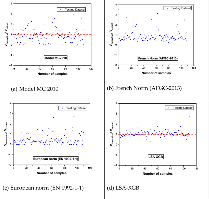
Results from existing shear capacity prediction models and comparison with the current study.
Table 5 shows the coefficient of regression (R2) and the theoretical to actual ratios of shear capacity. A high R2 value nearly 1, for instance, 0.9802 in LSA-XGB, shows that high predictability and ratio values closer to 1 imply more accuracy. The LSA-XGB model gives the highest overall performance with an R2 of 0.9802 and theoretical/actual ratio of 1.06, which suggests its predicted values are almost similar to the actual values. On the other hand, the other models, especially the European norm, have a large spread and lower accuracy, with the European norm model underpredicting, as evidenced by a ratio of 0.48. This analysis shows that there is a possibility of using machine learning techniques in structural engineering applications where accurate prediction of shear capacity is important, as compared to the use of traditional normative approaches.
Table 5 Comparison of different types of models.
The results of this study indicate that traditional models do not adequately capture the behaviour of UHPC beams, and future research should be directed toward refining or developing new shear capacity prediction methods that are more consistent with the unique structural characteristics of UHPC to ensure both safety and cost-effectiveness in design.
Since several parameters influence the shear behaviour of the UHPC beam, there is a critical issue in developing reliable and scalable modelling. To address this, an innovative GUI interface, as shown in Fig. 16, is integrated using the best-adopted model in the study. GUI development aims to generalize the state-of-the-art implementation of developed models for engineers and researchers. This framework can be helpful in the estimation of the shear strength of beams using their data. Further, engineers can make quick decisions by understanding the parameters influencing shear strength in real time for reliable problem-solving. This study integrates numerous libraries, including Pickle and Tkinter of the Python programming language. This interface can be scalable by integrating application-based modules into structural software.
Fig. 16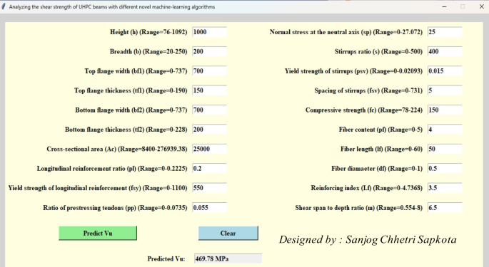
GUI for the prediction of shear strength of UHPC beam.