Non-semisimple anyons
The fusion rules governing anyons in our theory are closely related to SU(2)k Chern-Simons theory at level k = 2, in which each quasiparticle has a half-integer “q-deformed” spin quantum number, or q-spin, analogous to ordinary spin. Our fusion rules arise from the unrolled quantum group for \({\mathfrak{sl}}(2,{\mathbb{C}})\) with the quantum parameter set to an eighth root of unity27. This theory contains a vacuum state \({\mathbb{1}}\), and anyon types ψ, σ of q-spin 0, 1/2, and 1, respectively, as in the Ising theory, but also possesses new ‘non-semisimple’ anyon types removed in SU(2)2 Chern-Simons theory.
The non-semisimple theory retains additional anyon types that would have been removed in the traditional semisimplification process for SU(2)2. These include new anyon types α, indexed by non-half-integer real numbers, whose q-spins are no longer restricted to have half-integer values. The Hilbert space for the theory we propose augments Ising anyons by a single α-type anyon. However, to fully understand the fusion rules and constraints on the associated F-symbols, we must also consider q-spin 3/2 and 2 particles S3/2, and P2, all of which have traditional quantum trace zero at level k = 2.
The fusion rules relevant to our encoding are given by
$$\begin{array}{rl}\alpha \times {\mathbb{1}}=\alpha,&\alpha \times \sigma=(\alpha+1)+(\alpha -1),\\ \sigma \times \sigma={\mathbb{1}}+\psi,&\alpha \times \psi=(\alpha+2)+\alpha+(\alpha -2),\\ \sigma \times \psi=\sigma+{S}_{3/2},&\psi \times \psi={\mathbb{1}}+{P}_{2}.\end{array}$$
(2)
Observe that removing the anyon types S3/2 and P2 in the last line, as in the semisimplification procedure, results in the more familiar Ising fusion rules (1). A complete list of fusion rules can be found in ref. 21.
Consider the vector space \({{{\mathcal{H}}}}_{n}:={{{\mathcal{H}}}}_{\alpha ;{\sigma }^{2n}}\) consisting of a single type α-anyon and 2nσ-type anyons in a total q-spin state α. The fusion rules (2) imply that the space \({{{\mathcal{H}}}}_{n}\) is \(\left(\begin{array}{c}2n\\ n\end{array}\right)\)-dimensional and will contain our n-qubit topologically protected Hilbert space. The single qubit space \({{{\mathcal{H}}}}_{1}\) is encoded as \(\left\vert 0\right\rangle={({(\alpha,\sigma )}_{\alpha+1},\sigma )}_{\alpha }\), \(\left\vert 1\right\rangle={({(\alpha,\sigma )}_{\alpha -1},\sigma )}_{\alpha }\), where we denote the fusion of a pair of anyons ϕ and \({\phi }^{{\prime} }\) into a type t anyon using the notation \({(\phi,{\phi }^{{\prime} })}_{t}\). We can represent these states using fusion trees or by depicting the anyon labels grouped by ovals labeling the total q-spin.
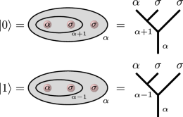
(3)
Such fusion trees give rise to bases for the Hilbert space of a collection of anyons in a fixed q-spin. An alternative single qubit Hilbert space is given by the states \(\left\vert {0}^{{\prime} }\right\rangle={(\alpha,{(\sigma,\sigma )}_{{\mathbb{1}}})}_{\alpha }\), \(\left\vert {1}^{{\prime} }\right\rangle=\left.\right({(\alpha,{(\sigma,\sigma )}_{\psi })}_{\alpha }\). The change of basis between these two bases is given by the matrix of F-symbols in the theory.
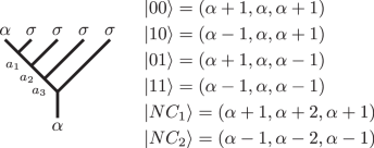
For multiple qubits, we must account for the noncomputational fusion channels \(\left\vert N{C}_{1}\right\rangle={({(\alpha,\sigma )}_{\alpha+1},\sigma )}_{\alpha+2}\), \(\left\vert N{C}_{2}\right\rangle={({(\alpha,\sigma )}_{\alpha -1},\sigma )}_{\alpha -2}\). The computational basis of n qubits is encoded into the fusion of α × σ×2n by having each 0 correspond to the fusion channel α × σ → α + 1 and each 1 to α × σ → α − 1 and each (α ± 1) × σ → α as illustrated below for n = 2,
(4)
where we encode the results of fusion as tuple (a1, a2, a3).
Note that while we use three anyons (α, σ, σ) to encode a single qubit, two qubits are encoded by adding just two additional Ising anyons (α, σ, σ, σ, σ). No additional α-type anyons are required in this multi qubit encoding.
Unlike the traditional framework of topological quantum computation, the non-semisimple theory gives rise to an inner product on the Hilbert space \({{{\mathcal{H}}}}_{n}\) that is not always positive definite27. This is an inherent property of the theory. Nevertheless, there are sectors within the theory where the computational space is positive definite. For α ∈ (2, 3), the inner product from ref. 27 is definite on the single qubit Hilbert space \({{{\mathcal{H}}}}_{1}\), but indefinite unitary more generally. For example, the two qubit space \({{{\mathcal{H}}}}_{2}\) has signature (+ , + , + , + , − , +), meaning that all basis vectors from (4) have norm + 1 except \(\left\langle N{C}_{1},N{C}_{1}\right\rangle=-\!1\). Remarkably, the signature for the computational subspace is always positive definite for α ∈ (2, 3) in the multi-qubit encoding, with indefinite signature only occurring on a portion of the noncomputational space. Braiding of anyons acts on the Hilbert space \({{{\mathcal{H}}}}_{n}\) by unitary transformations with respect to the indefinite metric. In order to preserve the Hilbert space \({{{\mathcal{H}}}}_{\alpha ;{\sigma }^{n}}\), we consider only those braids that take the α-type anyon to itself. This subset of braids is called the affine braid group and can be regarded as braids that are allowed to wrap around a stable, unmoved pole in the first strand.
Introduce real coefficients
$${{{\bf{B}}}}_{\alpha+1}:=\frac{\sqrt{2}}{-1+\cot \frac{\pi (\alpha+1)}{4}},\,\,\,{{{\bf{B}}}}_{\alpha -1}:=\frac{\sqrt{2}}{-1+\cot \frac{\pi \alpha }{4}},$$
(5)
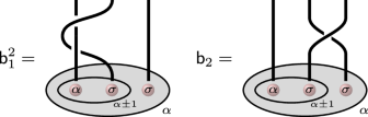
that arise when computing the inner product on the computational Hilbert space (see Section “Inner Products”). The braiding matrices are given on the computational space by
$$\begin{array}{l}{{\mathsf{b}}}_{1}^{2}=-q\,{\left({{\mathsf{b}}}_{1}^{\alpha \sigma \sigma }\right)}^{2}=\left(\begin{array}{cc}{q}^{\alpha }&0\\ 0&{q}^{-\alpha }\end{array}\right),\\ {{\mathsf{b}}}_{2}={q}^{-\frac{3}{2}}\,{{\mathsf{b}}}_{2}^{\alpha \sigma \sigma }={q}^{-1}\left(\begin{array}{cc}\frac{1+{q}^{2}}{1-{q}^{2\alpha }}&{q}^{-1}\frac{\sqrt{{{{\bf{B}}}}_{\alpha+1}}}{\sqrt{{{{\bf{B}}}}_{\alpha -1}}}\\ {q}^{-1}\frac{\sqrt{{{{\bf{B}}}}_{\alpha+1}}}{\sqrt{{{{\bf{B}}}}_{\alpha -1}}}&\frac{1+{q}^{2}}{1-{q}^{-2\alpha }}\end{array}\right)\end{array}$$
(6)
where we sometimes include the superscript to emphasize this single qubit encoding. The factors \({q}^{-\frac{3}{2}}\) and −q are global phases that were manually introduced to make the matrices special unitary.
An explicit computation shows that the matrices above satisfy the affine braid relation:
$${{\mathsf{b}}}_{1}^{2}{{\mathsf{b}}}_{2}{{\mathsf{b}}}_{1}^{2}{{\mathsf{b}}}_{2}={{\mathsf{b}}}_{2}{{\mathsf{b}}}_{1}^{2}{{\mathsf{b}}}_{2}{{\mathsf{b}}}_{1}^{2}$$
(7)
More generally, we have elementary braid generators \({{\mathsf{b}}}_{1}^{2}\), \({{\mathsf{b}}}_{2}\), …, \({{\mathsf{b}}}_{2n}\) acting on the space \({{{\mathcal{H}}}}_{n}\) with \({{\mathsf{b}}}_{i}\) swapping σ’s in position i and (i + 1) for i > 2.
Single qubit operations
Universality for single qubit operations is established by showing that braiding will produce a dense subgroup of SU(2). A standard approach from ref. 58 for showing density in SU(2) is to specify two non-commuting braids b1, b2 of infinite order.
If \(\alpha \in {\mathbb{R}}\setminus {\mathbb{Q}}\), then \({{\mathsf{b}}}_{1}^{2}\) and \({{\mathsf{b}}}_{2}\) are non-commuting and \({{\mathsf{b}}}_{1}^{2}\) has infinite order, but \({{\mathsf{b}}}_{2}\) has order four. However, \({{\mathsf{b}}}_{2}{b}_{1}{{\mathsf{b}}}_{2}^{-1}\) will have infinite order. Taking \({b}_{1}={{\mathsf{b}}}_{1}^{2}\) and \({b}_{2}={{\mathsf{b}}}_{2}{b}_{1}{{\mathsf{b}}}_{2}^{-1}\) gives two non-commuting matrices of infinite order; hence, braiding anyons for any irrational α will be dense for single qubit operations.
If \(\alpha \in {\mathbb{Q}}\), it takes more work to prove density. Here, we focus on the case \(\alpha=2+\frac{2}{5}\), where we have an explicit procedure for constructing low-leakage two-qubit entangling gates. For rational α, the braid \({({{\mathsf{b}}}_{1}^{\alpha \sigma \sigma })}^{2}\) no longer has infinite order, so we instead let \({b}_{1}=({{\mathsf{b}}}_{2}^{\alpha \sigma \sigma }){({{\mathsf{b}}}_{1}^{\alpha \sigma \sigma })}^{2}{({{\mathsf{b}}}_{2}^{\alpha \sigma \sigma })}^{2}\) and \({b}_{2}=\left({{\mathsf{b}}}_{2}^{\alpha \sigma \sigma }\right){b}_{1}{({{\mathsf{b}}}_{2}^{\alpha \sigma \sigma })}^{-1}\). b1 and b2 are not commuting, and they have infinite order if and only if b1 does. The eigenvalues of b1 at \(\alpha=2+\frac{2}{5}\) are \({e}^{\pm i(\arccos -\frac{\varphi }{\sqrt{2}})}\), where φ is the golden ratio, so this generator has infinite order as long as \(\arccos (-\frac{\varphi }{\sqrt{2}})\) is not a rational multiple of π. But all algebraic integers of order up to 4 that are twice the cosine of a rational multiple of π are classified in ref. 59. The order 4 algebraic integer \(-\sqrt{2}\,\varphi\) (a root of x4 − 6×2 + 4) is not included in the classified values. Hence, braiding of anyons is universal for single qubit operations when \(\alpha=2+\frac{2}{5}\).
From our encoding of multiple qubits, it is not immediately obvious that braiding will produce single qubit operations on each qubit in the multi-qubit space since we use just a single α-type anyon. However, by leveraging special braids acting locally on a single qubit, the proof of universality for single qubit operations above immediately extends to the multiqubit encoding, see Fig. 1.
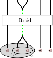
Fig. 1: An illustration of the braid J4 that acts diagonally on a single qubit away from the initial α-type particle.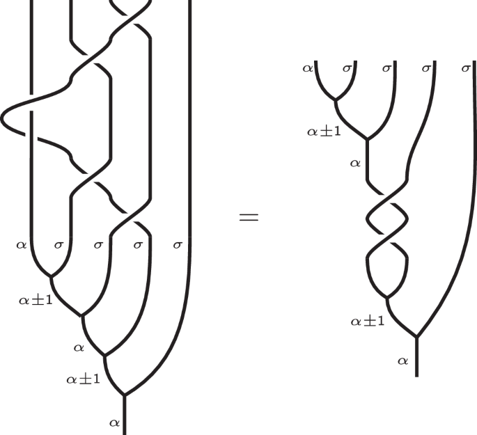
Because the topology of this braid is such that it can slide through the result of all previous fusions, this braid does nothing to qubits appearing earlier in the fusion tree. Topologically, it is the same as a simple twist acting on a qubit lower in the fusion tree.
In the basis of the two qubit space \({{{\mathcal{H}}}}_{2}\) for α × σ×4 from (4), single qubit operations can be performed on the first qubit using the affine braid generators
$${{\mathsf{b}}}_{1}^{2}={\left({{\mathsf{b}}}_{1}^{\alpha \sigma \sigma }\right)}^{2}\otimes {{\rm{Id}}}\oplus {\left({{\mathsf{b}}}_{1}^{\alpha \sigma \sigma }\right)}^{2}\\ {{\mathsf{b}}}_{2}={{\mathsf{b}}}_{2}^{\alpha \sigma \sigma }\otimes {{\rm{Id}}}\oplus \left({q}^{\frac{1}{2}}\,{{\rm{Id}}}\right)$$
(8)
Where \({{\mathsf{b}}}^{\alpha \sigma \sigma }\) refers to the matrices in (6). The single qubit operations on the second qubit can be achieved using
$${J}_{4} ={{\rm{Id}}}\otimes {\left({{\mathsf{b}}}_{1}^{\alpha \sigma \sigma }\right)}^{2}\oplus \left(\begin{array}{cc}{q}^{1-\alpha }&0\\ 0&{q}^{1+\alpha }\end{array}\right)\\ {{\mathsf{b}}}_{4} ={{\rm{Id}}}\otimes {{\mathsf{b}}}_{2}^{\alpha \sigma \sigma }\oplus \left({q}^{\frac{1}{2}}\,{{\rm{Id}}}\right)$$
(9)
where J4 is the composite braid \({{\mathsf{b}}}_{3}{{\mathsf{b}}}_{2}{{\mathsf{b}}}_{1}^{2}{{\mathsf{b}}}_{2}{{\mathsf{b}}}_{3}\). The first four basis vectors from (4) span the computational space, so J4 and b4 introduce no leakage in executing single-qubit operations.
The structure of (8) and (9) simplifies the compilation of single-qubit gates in the multi-qubit setting; knowing how to implement a gate on the first qubit automatically gives us a way of implementing it on the second qubit. For example, if a sequence of powers of \(({{\mathsf{b}}}_{1}^{2})\) and \({{\mathsf{b}}}_{2}\) generates the gate U ⊗ Id, U ∈ SU(2), then the same sequence in J4 and \({{\mathsf{b}}}_{4}\) will generate the gate Id ⊗ U.
Entangling gates
Given the ability to efficiently perform single-qubit operations on any qubit, achieving universal quantum computation also requires the implementation of entangling gates and controlling the leakage into the non-computational subspace. In many approaches to topological quantum computation, density is established across the entire anyonic Hilbert space, which implies density on the computational subspace. However, the challenge then shifts to constructing entangling gates that minimize leakage into non-computational states.
In our setting, it is more challenging to establish density on the full Hilbert space. In the two qubit setting, the 6-dimensional Hilbert space \({{{\mathcal{H}}}}_{2}\) has signature (+, +, +, +, −, +) and braiding produces a subgroup of SU(5, 1). Unlike the compact group SU(6), this group of matrices preserving an indefinite form is noncompact and the classification of its subgroups is much more complex. Very few techniques have been established for proving density in this setting23,60,61.
Rather than proving density for the entire Hilbert space \({{{\mathcal{H}}}}_{n}\), here we establish density only for the computational space. Our approach combines two techniques developed in the context of Fibonacci anyons. The first is a technique to apply controlled braiding where the state of a control qubit determines if a braid is executed on a target qubit following ideas from refs. 28,29,30. Second, we have a simple and efficient procedure for finding specific braids that produce diagonal phases with arbitrarily small leakage into the noncomputational space, adapting a procedure developed by Reichardt31 to the indefinite unitary setting. Together, these two strategies produce controlled phase gates.
The protocol for implementing controlled braid operations is built off the observation that σ × σ can fuse into the vacuum \({\mathbb{1}}\), or a ψ type anyon. Thus, braiding a pair of σ anyons through other anyons will produce a trivial operation when they are in the state \({\mathbb{1}}\), and a nontrivial operation when in state ψ.
Changing basis in the control qubit to the basis \(\left\vert {0}^{{\prime} }\right\rangle={(\alpha,{(\sigma,\sigma )}_{{\mathbb{1}}})}_{\alpha }\), \(\left\vert {1}^{{\prime} }\right\rangle=\left.\right({(\alpha,{(\sigma,\sigma )}_{\psi })}_{\alpha }\) (see Fig. 2), we give braids that act as the identity when the control channel is \({\mathbb{1}}\) and nontrivially when it is ψ. The gate implemented by this protocol is, by definition, a controlled gate in this basis. Transforming back to the original basis maintains the entanglement.
Fig. 2: An alternative basis for the two-qubit space \({{{\mathcal{H}}}}_{2}\) that is well suited for performing controlled operations.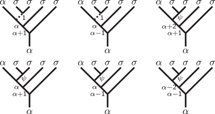
The first two σ-type anyons form the control pair. Braiding the pair through the other anyon types creates a controlled braiding operation that only acts nontrivially if the control pair fuses into the ψ channel. The subspace \({{{\mathcal{H}}}}_{2}^{\psi }\) consisting of states where the control qubit is in state ψ has basis given by the last four basis vectors that we denote by \(\left\vert {\psi }_{0}\right\rangle\), \(\left\vert {\psi }_{1}\right\rangle\), \(\left\vert {\psi }_{2}\right\rangle\), \(\left\vert {\psi }_{3}\right\rangle\).
For controlled braiding to entangle the computational space, we must identify low-leakage braids acting on the Hilbert space \({{{\mathcal{H}}}}_{2}^{\psi }\) corresponding to the anyon configuration (α, ψ, σ2) in a total q-spin state α. We focus on braids that preserve this space and become topologically trivial when ψ is replaced by the vacuum \({\mathbb{1}}\). Fix a basis of \({{{\mathcal{H}}}}_{2}^{\psi }\) consisting of the last four basis elements in Fig. 2 containing the fusion of σσ into a ψ state. We denote these by \(\left\vert {\psi }_{0}\right\rangle\), \(\left\vert {\psi }_{1}\right\rangle\), \(\left\vert {\psi }_{2}\right\rangle \left\vert {\psi }_{3}\right\rangle\), noting that \(\left\vert {\psi }_{0}\right\rangle\) and \(\left\vert {\psi }_{3}\right\rangle\) span the noncomputational space.
Our strategy to obtain low-leakage gate acting on \({{{\mathcal{H}}}}_{2}^{\psi }\) is to start with a gate w = U ⊕ V in SU(2) × SU(1, 1) and perform a sequence of braids to suppress the off-diagonal entries so that the resulting gate approximates a diagonal with a nontrivial phase on the computational subspace. Here SU(2) acts on the space spanned by \(\left\vert {\psi }_{0}\right\rangle\), \(\left\vert {\psi }_{1}\right\rangle\), and SU(1, 1) acts on the space spanned by \(\left\vert {\psi }_{2}\right\rangle\) and \(\left\vert {\psi }_{3}\right\rangle\), where \(\left\vert {\psi }_{1}\right\rangle\) and \(\left\vert {\psi }_{2}\right\rangle\) span the computational space.
For matrices U ∈ SU(2), Reichardt gave a procedure for leveraging a specific diagonal matrix \({D}_{(2)}=\left(\begin{array}{cc}{e}^{\frac{i3\pi }{5}}&0\\ 0&1\\ \end{array}\right)\) to produce a sequence of unitaries Uk whose off-diagonal entries decrease exponentially [ref. 31, Eq. 3]. Reichardt used a slightly different definition of D(2), although the procedure works the same. The recursive sequence is given as follows:
$${U}_{0} =U\\ {U}_{k+1} ={U}_{k}{D}_{(2)}{U}_{k}^{{\dagger} }{D}_{(2)}^{3}{U}_{k}{D}_{(2)}^{3}{U}_{k}^{{\dagger} }{D}_{(2)}{U}_{k}$$
(10)
One computes that the off-diagonal entries satisfy ∣〈0∣Uk+1∣1〉∣ = ∣〈0∣Uk∣1〉∣5, and hence that \(| \langle 0| {U}_{k}| 1\rangle |=| \langle 0| U| 1\rangle {| }^{{5}^{k}}\). For unitary matrices, the off-diagonal entries are less than or equal to 1, so iterating this procedure suppresses the off-diagonal entries to arbitrary accuracy. Note that, even though the sequence in (10) has an exponential length in k, the off-diagonal terms go to zero doubly exponentially. While it is not possible to control the phases of the resulting diagonal matrix, one can still use the algorithm to produce entangling gates62.
Recall that matrices V in SU(1, 1) have unit determinant and satisfy V†JV = J where \(J=\left(\begin{array}{cc}1&0\\ 0&-1\\ \end{array}\right)\). The general form of such a matrix is \(V=\left(\begin{array}{cc}\alpha &\beta \\ {\beta }^{*}&{\alpha }^{*}\\ \end{array}\right)\) where ∣α∣2 − ∣β∣2 = 1. Unlike the case of SU(2), the off-diagonal entries β need not have a norm less than or equal to 1, so Reichardt’s algorithm does not immediately apply. However, for V ∈ SU(1, 1) and \({D}_{(1,1)}=\left(\begin{array}{cc}1&0\\ 0&{e}^{\frac{i3\pi }{5}}\\ \end{array}\right)\), and setting
$${V}_{0} =V\\ {V}_{k+1} ={V}_{k}{D}_{(1,1)}{V}_{k}^{-1}{D}_{(1,1)}^{3}{V}_{k}{D}_{(1,1)}^{3}{V}_{k}^{-1}{D}_{(1,1)}{V}_{k}$$
(11)
a direct computation shows that ∣〈0∣Vk+1∣1〉∣ = ∣〈0∣Vk∣1〉∣5. Thus, if V can be found with ∣〈0∣V∣1〉∣ SU(1, 1) with exponentially suppressed off-diagonal terms.
Combining these two constructions, for D = D(2) ⊕ D(1, 1), and W = U ⊕ V ∈ SU(2) ⊕ SU(1, 1), the recursive sequence
$${W}_{0} =W\\ {W}_{k+1} ={W}_{k}D{W}_{k}^{-1}{D}^{3}{W}_{k}{D}^{3}{W}_{k}^{-1}D{W}_{k}$$
(12)
then in the ordered basis \(\{\left\vert {\psi }_{0}\right\rangle,\left\vert {\psi }_{1}\right\rangle,\left\vert {\psi }_{2}\right\rangle,\left\vert {\psi }_{3}\right\rangle \}\) we have \(| \langle {\psi }_{0}| {W}_{k}| {\psi }_{1}\rangle |=| \langle {\psi }_{0}| W| {\psi }_{1}\rangle {| }^{{5}^{k}}\) and \(| \langle {\psi }_{2}| {W}_{k}| {\psi }_{3}\rangle |=| \langle {\psi }_{2}| W| {\psi }_{3}\rangle {| }^{{5}^{k}}\). In particular, if ∣〈ψ0∣W∣ψ1〉∣ ∣〈ψ2∣W∣ψ3〉∣
This is where our specific choice α = 2 + 2/5 enters our analysis. For this value of α, a direct computation shows that \({({{\mathsf{b}}}_{1}^{\alpha \psi \sigma \sigma })}^{4}={D}_{(2)}\oplus {D}_{(1,1)}\). It remains to identify a braid W of the form W = U ⊕ V that is topologically trivial when the strand labeled ψ is removed and has small leakage term ∣〈ψ2∣W∣ψ3〉∣ \({\left({{\mathsf{b}}}_{2}^{\alpha \psi \sigma \sigma }\right)}^{2}\) but when α = 2 + 2/5, \({\left({{\mathsf{b}}}_{2}^{\alpha \psi \sigma \sigma }\right)}^{2}\) has non unitary leakage ∣〈ψ0∣W∣ψ1〉∣ ~ 1.943 > 1. Another candidate is the restriction of the braid \(W:={\left({{\mathsf{b}}}_{2}^{\alpha \psi \sigma \sigma }\right)}^{2}{\left({{\mathsf{b}}}_{1}^{\alpha \psi \sigma \sigma }\right)}^{2}{\left({{\mathsf{b}}}_{2}^{\alpha \psi \sigma \sigma }\right)}^{2}{\left({{\mathsf{b}}}_{1}^{\alpha \psi \sigma \sigma }\right)}^{2}{\left({{\mathsf{b}}}_{2}^{\alpha \psi \sigma \sigma }\right)}^{-2}\) from Fig. 3 to the four-dimensional space \({{{\mathcal{H}}}}_{2}^{\psi }\); it has the form W = U ⊕ V, where U ∈ SU(2) and V ∈ SU(1, 1) and acts as the identity if the control channel is in the vacuum state.
Fig. 3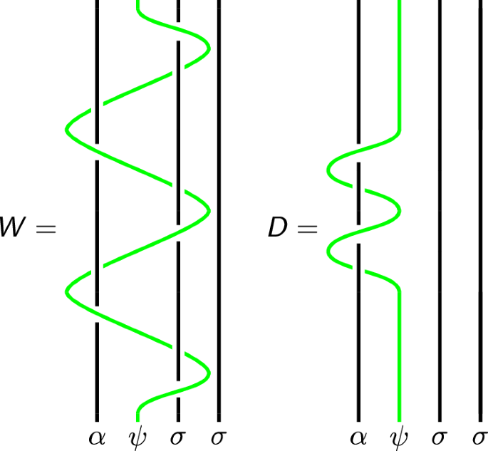
The braids W and D. Note that if the control strand (green) is the vacuum, the braids are topologically trivial.
W has leakage terms ∣〈ψ0∣W∣ψ1〉∣ ~0.832 ∣〈ψ2∣W∣ψ3〉∣ ~0.904
$${{\mathsf{b}}}_{2}{{\mathsf{b}}}_{1}{{\mathsf{b}}}_{2}{{\mathsf{b}}}_{1}^{-1}{{\mathsf{b}}}_{2}^{-1}{{\mathsf{b}}}_{1}{{\mathsf{b}}}_{2}{{\mathsf{b}}}_{1}{{\mathsf{b}}}_{2}{{\mathsf{b}}}_{1}^{2}{{\mathsf{b}}}_{2}$$
has initial unitary and non-unitary leakage terms with norms ~0.286 and ~0.285, respectively; these norms both reduce to ~1.914 × 10⁻³ upon applying Reichardt’s prescription once, and to 2.565 × 10⁻¹⁴ after a second application. This modification of Reichardt’s algorithm produces an approximate diagonal, non-leaking gate. We just have to verify that it doesn’t act like (a multiple of) the identity on the computational space. This is easy to verify numerically; analyzing the third iteration of Reichardt’s sequence (12) with starting braid W, we see that the diagonal gate acts on the computational space as diag\(({e}^{i{\theta }_{1}},{e}^{i{\theta }_{2}})\) where θ1 ~ −1.772 and θ2 ~ −1.682. The doubly exponential convergence rate ensures that further iterations will not meaningfully change these values62.