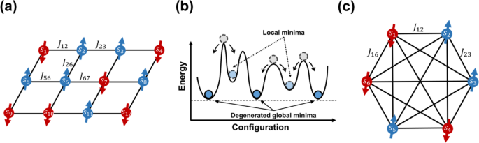
Number partitioning problem (2-NPP)
Using the model described above, we aim to deepen the understanding of the outcomes of p-computing and validate our p-computing model by focusing on the NPP, which is frequently termed ‘the easiest hard problem’ using the sampled random number generator described in the “Methods” section. It aims to redistribute a set of K elements, NU containing {n1, n2, …, nK}, into two subsets NA and NB, such that the difference (D) between sums of elements in sets A and B is minimized, which is described in Fig. 3a.
$$\:D=\left|\sum_{{n}_{i}\in\:{N}_{\text{A}}}{n}_{i}-\sum_{{n}_{j}\in\:{N}_{\text{B}}}{n}_{j}\right|\:\:\:\:\:\:\:\:\left({n}_{i},{n}_{j}\in\:{N}_{\text{U}}\:\right)$$
(5)
Fig. 3
(a) Schematic of flow of number partitioning problem. (b) The flow of problem implementations from mapping with construction of the Hamiltonian.
As the K increases, the possible combinations of subsets NA and NB grow exponentially. With a slight modification to Eq. 5, D can be expressed as:
$$\:D=\left|\sum_{{n}_{p}\in\:{N}_{\text{A}}}{n}_{p}\times\:(+1)+\sum_{{n}_{q}\in\:{N}_{\text{B}}}{n}_{q}\times\:(-1)\right|=\left|\sum_{i=1}^{K}{n}_{i}{s}_{i}\:\right|\:\left\{\begin{array}{c}{s}_{i}=\:+1\:\left(\text{i}\text{f}\:{n}_{i}\in\:\text{A}\right)\:\\\:{s}_{i}=\:-1\:\left(\text{i}\text{f}\:{n}_{i}\in\:\text{B}\right)\end{array}\right.$$
(6)
Identifying a subset with the minimum D is equivalent to finding a subset with the minimum D2 enabling the use of the energy cost function: \(\:{E}_{\text{N}\text{P}\text{P}}\left(\overrightarrow{s}=\left({s}_{1},{s}_{2},\ldots\:,{s}_{K}\right)\right)={\left(\sum\:_{i=1}^{K}{n}_{i}{s}_{i}\right)}^{2}\). Once the energy function of the COP is formulated using a suitable algorithm, it must be mapped onto the p-computing framework. The overall procedure for this transformation is illustrated in Fig. 3b. The energy minimization process involves taking the derivative of the energy \(\:{E}_{\text{N}\text{P}\text{P}}\) with respect to the variables (si) and orienting the system towards a negative energy gradient, resulting in \(\:{J}_{ij}=-2{n}_{i}{n}_{j}\left({1-\delta\:}_{ij}\right)\) and hi = 0 in Eq. 3.
Here we define the set NU = {2, 10, 13, 14, 23, 24, 28, 31, 36, 41, 47, 51, 59, 69, 72, 73} containing 16 elements as a test example. Figure 4a illustrates the total number of possible combinations as a function of D from the NU. For instance, in this example, only one combination exists for D = 593 (\(\:{N}_{\text{A}}={N}_{\text{U}},\:\:{N}_{B}=\varnothing\:)\:\), whereas D = 15 permits 310 possible cases out of a total of 216/2 cases. And one can check that the optimal solution is D = 1 (for example, \(\:{N}_{\text{A}}=\left\{2,\:10,\:14,\:31,\:47,\:51,\:69,\:73\right\},\:{N}_{B}=\left\{13,\:23,\:24,\:28,\:36,\:41,\:59,\:72\right\}\)). Our simulation shows a very similar pattern when each p-bit operates independently (i.e., Io = 0), leading to completely random fluctuations among the bits. Figure 4b illustrates the count of combinations of the simulation result with Io = 5 × 10⁻² in decimal notation. The graph clearly indicates that combinations resulting in D = 1 or other small values (e.g., 3, 5, 7, etc.) exhibit relatively high probabilities of occurrence. Moreover, we observed how the p-bits’ states fluctuate between different combinations while maintaining the same energy (D) due to the system’s degeneracy in the ground state. Without perfect clamping of p-bit, there is always possibility of bits to move to the excited states, causing the system to oscillate between excited and ground states, thus altering its combinations accordingly.
During the optimization process, it is important to avoid getting trapped in the local minima. P-computing follows the inverse temperature (Io ~ 1/T) dependent property, which is analogous to system’s temperature in simulated annealing28,29. The appropriate annealing path can reduce the likelihood of getting trapped in local minima. In general, the system begins with a low initial value of Io, allowing the p-bit configurations to explore a wide range of states and thereby reducing the risk of becoming trapped in local minima. Gradually increasing Io over time guides the system toward convergence on a more optimal solution. To investigate the influence of the annealing path, we applied the formula \(\:{I}_{\text{o}}\left(t\right)={I}_{0}+({I}_{\text{f}}-{I}_{0})\times\:\text{m}\text{i}\text{n}\left\{1,{\:\left(\frac{t}{{t}_{\text{o}}}\right)}^{P}\right\}\), where \(\:{I}_{0}\) represents the initial value of the annealing coefficient, \(\:{I}_{\text{f}}\) denotes the final value of it, and \(\:{t}_{\text{o}}\) is the total number of annealing iterations. The first aspect studied was the annealing rate. We set the trajectory of a linear annealing path with to values of 1, 103, 104, 105, and 106, where P = 1, I0 = 0, and If = 5 × 10⁻². After the annealing process is completed, we measured 500 iterations and recorded the most probable state. This process was repeated 1,000 times, and the sum of all these results is shown in Fig. 4c. As the annealing rate slows down (i.e. to increases), the probability of convergence to the ground state (D = 1) rises. However, when the rate surpasses a certain threshold (to ~ 105), the probability of reaching the ground state saturates. This observation suggests the existence of an optimal annealing rate, which can achieve the fastest problem-solving performance.
The other aspect examined was the influence of the shape of the annealing path, which is decided by the polynomial power (P). We tested values of P at 10−2, 10−1, 1, 10, and 102, as the results shown in Fig. 4d. In these tests, I0 = 0, If = 5 × 10⁻², and to was fixed at 106. In addition, we performed the annealing process 1,000 times, recording the most probable state at each test. The results clearly indicate that cases with P = 10−2 and 10−1 are more prone to getting trapped in local minima (D = 3, 5, 7, etc.) compared to others, suggesting that rapid annealing at the initial stage can lead to local minima entrapment. For P > 1, the outcomes are generally consistent; however, the probability of reaching the ground state slightly decreases when P = 102, indicating that overly abrupt annealing even in the later stages can also increase the chances of local minima entrapment.
Fig. 4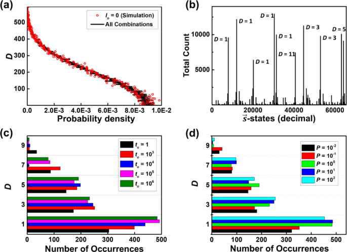
(a) The total number of possible combinations as a function of D in the test example. (b) Results of computation with the combinations represented in decimal notation. (c) The total count of each D value (1, 3, 5, 7, 9) in 1,000 repeated tests with to being 1, 1,000, 10,000, and 100,000 when P = 1 (linear annealing), I0 = 0 and If = 0.05. (d) The total count of each D value (1, 3, 5, 7, 9) across 1,000 repeated tests with P being 10−2, 10−1, 100, 101, 102 when to = 1,000,000, I0 = 0 and If = 0.05.
Next, we addressed the partition problem on a larger scale, aiming to identify the optimal subsets NA and NB from a set of 1,024 randomly selected numbers (|NU| = 1,024) ranging between 100 and 100,000, with no duplicates (see Supplementary Material). The total sum of all elements was 50,989,089, with the minimum achievable difference (D) being 1 in the actual solution. We employed a polynomial annealing approach with parameters n = 10, Io = 0, and If = 7.5 × 10⁻⁵ over 100,000 annealing iterations. Given that the total number of possible configurations for this set is approximately 10308, it is practically impossible to solve using current von Neumann techniques. As shown in Fig. 5a, D tends to reach lower values as the iteration progresses. The subsets NA and NB that yielded the lowest D (= 1) clearly correspond to the global minimum, with \(\:\sum\:_{{n}_{i}\in\:{N}_{A}}{n}_{i}\) = 25,494,544 and \(\:\sum\:_{{n}_{i}\in\:{N}_{B}}{n}_{i}\) = 25,494,545 (see Supplementary Material) from our simulation results. Figure 5b presents the result of the repeated tests. Their statistics show that, despite the calculations not achieving the global minima, most tests (~ 78.8%) were reasonably optimized and settled in acceptable local minima (lower than the smallest random number).
Fig. 5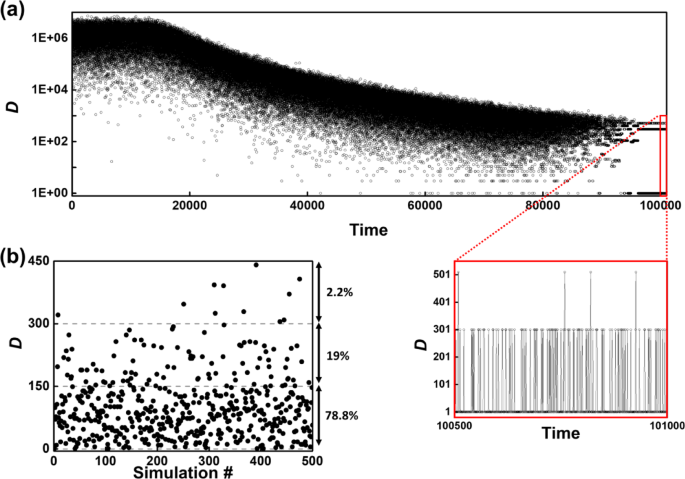
(a) The trajectory of D difference between the sums of elements in sets A and B over iterations. (b) The distribution of the D after 500 runs of 1024-bit simulation, demonstrating that the system is reasonably optimized and stabilized within acceptable local minima.
Multiway number partitioning problem (k-NPP)
Next, we performed simulations on k-way number partitioning problem (k-NPP), as an extension of the 2-NPP using the model we proposed in the Theoretical Frameworks section. In k-NPP, the objective can vary depending on the intended purposes: minimizing the difference between the largest sum (∑Smax) and the smallest sum (∑Smin), maximizing ∑Smin, or minimizing ∑Smax. While these objectives are identical for k = 2 (2-NPP), they can be diversified for k ≥ 3. By incorporating a refined penalty term, which can be seen as perturbation to the original Hamiltonian, it is possible to achieve precise control over the partitioning. However, a detailed discussion of this refinement is beyond the scope of this paper. Therefore, we focus specifically on the multiway number partitioning, where the primary objective is to minimize the difference between ∑Smax and ∑Smin.
We first applied the proposed p-trit concept, as introduced in the Theoretical Frameworks section, to the 3-way number partitioning (3-NPP) problem using the previously defined number set NU for the 2-NPP case. Figure 6a presents the normalized probability density function (PDF(D)) from the NU set, obtained through both exhaustive search and simulation (Io = 0). In the 3-NPP, the number of possible combinations increases significantly compared to the 2-NPP. For example, there are 1,240 possible states for D = 1, whereas the number of cases rises to 64,696 for D = 150 out of a total of 316/3. This highlights the substantial increase in complexity and variability in comparison to the 2-NPP. Figure 6b and c display the results with Io = 0.01. The most probable state, represented as 7,159,447 in decimal notation (= 0111110201220201(3)), exhibits the highest peak in Fig. 6c. This state corresponds to the subsets {2, 28, 36, 59, 72}, {10, 13, 14, 23, 24, 41, 73}, and {31, 47, 51, 69}. It achieves a difference (D = ∑Smax – ∑Smin) of 1, satisfying the ideal equipartition goal for the 3-NPP by minimizing D.
Fig. 6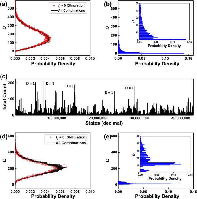
(a) The number of possible combinations as a function of D in the p-trit example and the simulation results when Io = 0. (b) The probability density of p-trit simulation with Io = 0.01. (c) Results of 3-level p-computation with the combinations represented in decimal notation. (d) The number of possible combinations as a function of D in the p-quintet example and the simulation results when Io = 0. (e) The probability density of p-quintet simulation with Io = 0.01.
We subsequently applied the 5-way number partitioning (5-NPP) to the set of NU = {38, 37, 56, 68, 25, 54, 31, 48, 96, 7, 22, 85, 74}, where the ideal value for each 5 subset is as close as \(\:\sum\:{N}_{\text{U}}/5=128.2\). The normalized PDF(D), as shown in Fig. 6d, clearly shows the tendency of more complexity and variability than lower-level NPP problems. For example, there are 24 possible states for the global minima D = 2, whereas the number of cases rises to 1,598,512 for D = 218 out of a total of 513/5. Figure 6e shows the results obtained with Io = 0.01 and 100,000 iterations. The most probable state, represented by the decimal notation 955,882,115 (corresponding to the 5-base number 3424201211430(5)), exhibits the highest peak. This state corresponds to the following subsets: {54, 74}, {31, 96, 7}, {56, 25, 48}, {37, 85}, and {37, 68, 22}. The difference between ∑Smax (= 134) and ∑Smin (= 122) is 15, which represents one of the local minima but is reasonably optimized. It is also noteworthy that Fig. 6e shows additional peaks in the region where D
If a multi-level system can be physically implemented, it could be realized without additional circuitry. The implementation of a p-trit can be achieved using a photon (optical oscillator30,31 with three states (+ polarization, –polarization, or no light) or a nonlinear oscillator32,33 with phases of 0°, 120°, and 240° as the information unit. Another approach involves utilizing a spin glass system34,35, which consists of three nanomagnets with easy axes oriented 120o apart, where two are freely oriented and one is fixed. Of the four possible configurations, three have the same low energy level, and by introducing a low energy barrier, these three can be made metastable, allowing for inter-fluctuations. Recent research also suggests that probabilistic transitions can occur in Kagome lattice structures36,37, potentially enabling p-trit and p-computing based on a 3-fold Kagome lattice system.