This study presents a novel framework of disaster prediction, integrating federated learning and blockchain technology, called mTCN-FChain, shown in Fig. 1. This methodology models sequential data from diverse sources, including earthquake, tsunami, and flood datasets, with TCN. Federated learning allows decentralized training across edge devices while preserving data privacy and enabling collaborative learning. The process is made secure through model updates encryption and authenticity verification by digital signatures along with an immutable ledger for traceability and accountability purposes. The proposed framework also embeds WNLs for data transmission and processing. The aggregate global model that validated on the level of blockchain would be deployed onto edge devices then conduct real-time disaster prediction based on greater precision. This encompassing methodology supports secure, scaled, and privacies-preserving disaster monitoring with prediction for hazardous regions.
Fig. 1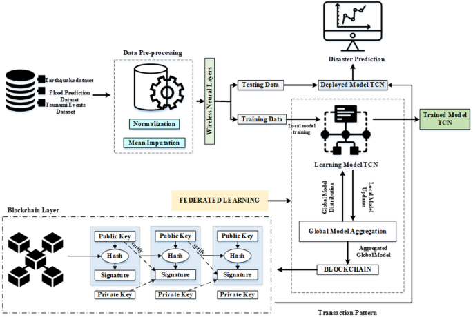
Workflow of proposed method mTCN-FChain.
Data collection
This study uses real-time data from the IoT sensors; three datasets were used to make predictions. Earthquake Dataset spans from 2001 to 2023 which provides a magnitude and location for forecasting purposes. Flood Dataset comprises 50,000 records with details of the parameters from the hydrological and meteorological sensors. These parameters will be analyzed in predicting flood risk. The Tsunami Events Dataset, which contains more than 2000 records, collects wave height and source event data from oceanographic sensors and together supports accurate and real-time disaster prediction models.
Earthquake dataset
The earthquake dataset22 comprises 782 cases and seismic events from January 1, 2001, to January 1, 2023; earthquakes’ attributes include the magnitude, date, time, latitude, longitude, depth, and CDI, MMI, and SIG indicators. Event risk categorization is done based on its alert levels (“green,” “yellow,” “orange,” “red”) while a tsunami flag indicates ocean events. Other parameters like NST, GAP, MAGTYPE also help in making a result more reliable and geographical information gives more background information. Due to its highly featured and real-time nature, this dataset is used in the study for pattern recognition and earthquake prediction using TCNs and for localized training in federated learning. They include scalability, accuracy and privacy and therefore, it is appropriate to be used in efficient disaster prediction. Summary of earthquake dataset parameters were given in Table 2.
Table 2 Summary of recent significant earthquake events with key parameters (2023).Flood prediction dataset
There are 50,000 rows in the flood prediction dataset23 and 21 numeric features that include variables like Monsoon Intensity, Deforestation, Urbanization, Drainage Systems, and Flood Probability as the target variable. With no missing value and all the data being of integer type, this dataset will prove ideal for use with regression models without much data preprocessing. This work provides a detailed overview of flood causes, which include climate change, human activities, and infrastructural issues. Utilizing this dataset will enable the proposed mTCN-based model to analyze complex interactions accurately, enhancing the precision of flood prediction and supporting proactive strategies for disaster management. Summary of flood prediction dataset parameters were given in Table 3.
Table 3 Key environmental factors for flood prediction: sample dataset overview.Tsunami events dataset (1900–Present)
The Tsunami Events Dataset (1900–Present)24 includes comprehensive information on more than 2000 tsunamis which occurred in the whole world, as well as their feature, based on which the events have occurred, their date and time, location, magnitude, as well as death and injuries count. It is further supplemented with bathymetry data, which facilitate the depiction of the tsunami wave movement prognosis. Tsunami data is important for identifying causes, impacts and temporal distribution, making this dataset particularly useful for tsunami studies, planning and intervention. The broad scope and open access strengthen the potential for constructing better predictive models, which substantively enriches disaster risk analysis and decision-making in this investigation. Summary of Tsunami events dataset parameters were given in Table 4.
Table 4 Tsunami events dataset (2023): magnitude, timing, and Impact.Data pre-processing
This study utilizes normalization to standardize numerical features within datasets, and mean imputation is applied in missing value imputation to replace missing data with mean value of observed data. These pre-processing steps help to check the quality and completeness of the data fed into the system. They are specifically required when training the TCNs. The workflow of data pre-processing in shown in Fig. 2.
Fig. 2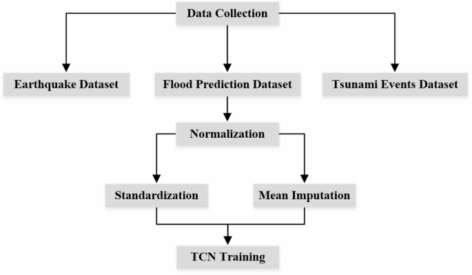
Workflow of data pre-processing.
Normalization
Normalization (or standardization) is a technique applied to scale numerical data into a constant range, hence making it easier for machine learning models to learn and perform well. Normalization usually scales the data to a [0, 1] range, while standardization transforms the data so that it has mean 0 and a standard deviation of 125. When features such as magnitude due to an earthquake, flood probability, and tsunami impact have varying numerical ranges, the appropriate application of this technique is important in TCNs. For instance, the magnitude of an earthquake can be between 1 and 9, while the probability of a flood is between 0 and 100. This would make the model place greater emphasis on the probability of a flood since it is the larger scale. Standardization is done using the following Eq. (1).
$$\:{X}_{standardized}=\frac{X-\mu\:}{\sigma\:}$$
(1)
where \(\:X\) is the original value, \(\:\mu\:\) is the mean of the feature, and \(\:\sigma\:\) is the standard deviation of the feature. This process makes it possible for all features to get into a similar scale which makes the model more efficient and not to be biased toward large-value features.
Missing value imputation by mean imputation
Missing values in a dataset may result in incorrect predictions or incomplete models. Mean imputation is one of the most common techniques for dealing with missing data, where missing values are replaced by the mean of the observed values in the feature26. This is quite valuable in the case of numerical features such as the probability of a flood or the magnitude of a tsunami, where the data may be missing due to reporting errors or other reasons. Mean imputation is simple and helps retain the overall distribution of the data. The formula for mean imputation is given in Eq. (2).
$$\:{X}_{imputed}=\frac{\sum\:{X}_{observed}}{N}$$
(2)
where, \(\:{X}_{imputed}\) is the value used to replace the missing data, \(\:\sum\:{X}_{observed}\) is the sum of all the data points that are not missing; n is the number of data points that are not missing.
Wireless-aware neural layer (WNLs)
WNLs are layers that improve wireless data transmission by using neural network models to dynamically adapt to network conditions such as signal strength, bandwidth, and congestion. In this work, WNLs are applied after data collection, optimizing the transmission process before the data reaches edge nodes. WNLs reduce packet loss through error-correcting codes and adaptive retransmission mechanisms, ensuring data integrity even in noisy environments. They minimize latency through dynamic transmission rates and critical data prioritization in order to prevent network congestion. Intelligent routing is implemented so that WNLs predict optimal paths and make selections based on real-time network metrics for robust data delivery. Once data reaches the edge nodes, it is subjected to lightweight preprocessing and initial analysis using the Lightweight TCN. The working of WNLs is given in Fig. 3.
Fig. 3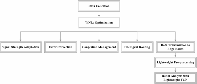 Temporal convolutional networks (TCNs)
Lightweight TCNs mechanism is intended to efficiently process time-series data, especially in resource-constrained environments like those with limited computational resources and network bandwidth27. Lightweight TCNs have several layers with unique contributions toward the overall functionality of the model. This section expands on the role of each layer, with special emphasis on how they work together to process time-series data for real-time disaster prediction. The architecture of TCN is shown in Fig. 4. The Input Layer is the first contact point with the model. The time-series data is received and usually pre-processed by WNLs. It plays a critical role in this step as they optimize the data transmission from the IoT devices to the edge nodes by reducing noise and only transmitting relevant information. This pre-processing step improves the quality of the input data, which is very important for proper predictions. The convolutional layers are the core component of TCNs, and they are designed to extract features from the input time-series data.
First layer: This layer uses causal convolutions, with specified kernel size. The causal convolutions do ensure that the predictions produced for time \(\:t\) depend only on inputs up to previous time steps while keeping their temporal order necessary for predictions. Mathematically this can be expressed as Eq. (3).
$$\:{y}_{t}=\sum\:_{i=0}^{k-1}{w}_{i}\cdot\:{x}_{t-i}$$
(3)
where \(\:{y}_{t}\) is the output at time \(\:t\), \(\:{w}_{i}\) are the weights of the convolution kernel, and \(\:x\) represents the input sequence.
Fig. 4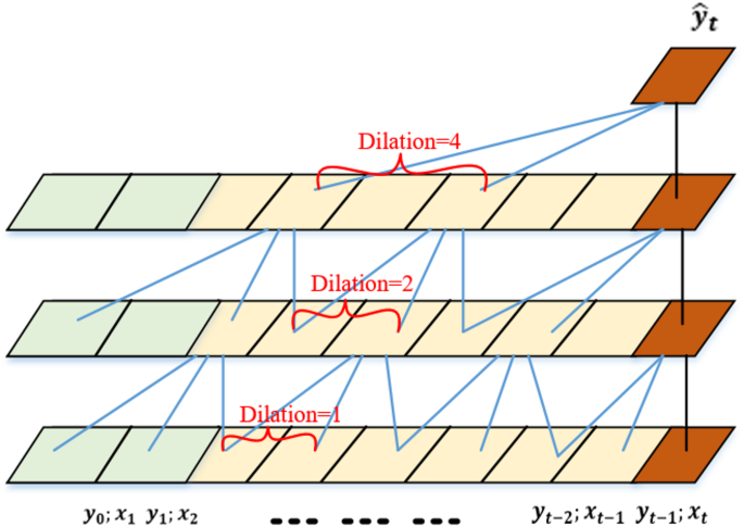
Dilated convolutional layers: Following layers apply dilated convolutions with increasing dilation rates. Dilation allows the network to expand its receptive field without significantly increasing the number of parameters. For example, setting dilation rates \(\:d=\text{1,2},4,\) each layer processes inputs with different receptive fields given in Eq. (4).
$$\:{y}_{t}=\sum\:_{i=0}^{k-1}{w}_{i}\cdot\:{x}_{t-d\cdot\:i}$$
(4)
This way, it can understand dependencies across longer time spans effectively without losing computational efficiency. After feature extraction, TCN computes an anomaly score to determine whether the current observation significantly deviates from the expected behavior. The TCN utilizes a 96-hour receptive field, which is intended to capture long temporal dependencies typical of disaster events such as slow pressure declines ahead of a flood or seismic precursors in earthquakes, which improve early prediction capabilities and false alarm rates.
Localized anomaly detection
Edge-based TCNs can perform local anomaly detection, where it able to identify any irregular behavior or pattern within time-series data coming from a sensor or other IoT device. It processes the incoming streams of data and looks for patterns that may hint at a possible disaster, it can be a temperature rise, uncharacteristic seismic activity, or unusual levels of rainfall. This model uses causal convolutions in order to have predictions based on past data therefore, maintains the necessary temporal integrity required to be correct for any kind of prediction. Mathematical representation of an anomaly score can be computed as Eq. (5).
$$\:Anomaly\:Score=\left|{y}_{t}^{predicted}-{y}_{t}^{actual}\right|$$
(5)
Here, \(\:{y}_{t}^{predicted}\) is the predicted value from the TCN model, and \(\:{y}_{t}^{actual}\:\)is the actual observed value. If this score exceeds a predefined threshold \(\:\tau\:\), an alert can be triggered for further investigation. For every convolutional layer, the non-linear activation functions such as ReLU are applied. Such functions allow a model to introduce non-linearity and therefore capture complex patterns from the data. The definition of the ReLU function can be given by Eq. (6).
$$\:f\left(x\right)=max\left(0,x\right)$$
(6)
This non-linearity is crucial for enabling TCNs to model intricate relationships within time-series data. Residual Blocks are introduced after some of the convolutional layers to further improve learning within deeper networks. The residual block of TCN is shown in Fig. 5.
Fig. 5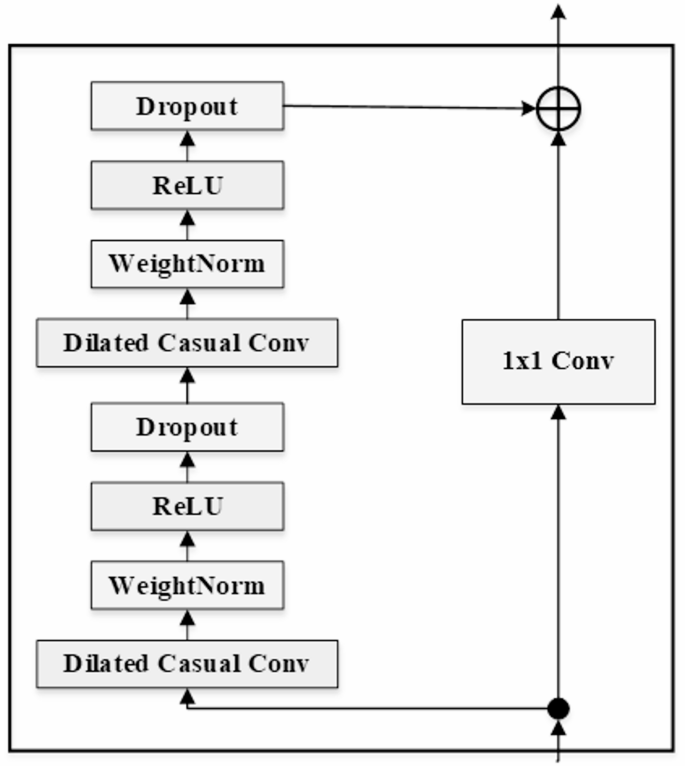
A residual block adds outputs of convolutional layers with their corresponding inputs which is given in Eq. (7).
$$\:{y}_{t}^{residual}=F\left({x}_{t}\right)+{x}_{t}$$
(7)
where, \(\:F\left({x}_{t}\right)\) is the output of a set of convolution operations applied to the input \(\:{x}_{t}\). This design helps reduce problems of vanishing gradients, hence training better and deeper networks without performance degradation. The Output Layer generates predictions given the features which have been passed through previous layers. For a disaster prediction problem, this output is the probabilities of certain events (such as floods or earthquakes) happening in a given timeframe. The output can be written as Eq. (8).
$$\:P\left(events|features\right)=softmax\left({W}_{y}+b\right)$$
(8)
where \(\:W\) are the weights learned during training, \(\:y\) represents the output from the last hidden layer, and \(\:b\) denotes a bias term.
Federated learning workflow for disaster prediction
In this study, Federated Learning (FL) is applied to develop a disaster prediction model using multiple edge devices with different disaster datasets, for instance, handling tsunami, flood, and earthquake disasters. This will ensure the development of a robust global model, capable of making predictions of all types of disaster, and thus ensuring scalability, preservation of privacy, and adaptability in different disaster scenarios.
Local mTCN models: Each edge node trains a lightweight TCN, mTCN is trained on its assigned disaster dataset. This localized scheme allows each of the models to specialize in disaster type, meaning it can then better predict under certain conditions in an earthquake event, flood or tsunami. Due to the naturally non-IID nature of data associated with disasters between nodes (i.e., coastal nodes handling tsunami data versus inland nodes handling flood data), the challenges related to model convergence can be addressed through normalization of data sets, as well as balancing the weights that are aggregated during model fusion. This type of heterogeneity is part of the real-life deployment, as well as a key aspect when creating a robust and generalized global model. Local models perform short-term trend analysis to detect immediate disaster signals like seismic or flood indicators, enabling timely alerts. They also capture long-term patterns such as seasonal or oceanographic trends to improve disaster forecasting and preparedness.
Federated learning workflow
Federated learning is used to enable the models on edge devices to collaboratively train a global model in a distributed manner without transferring sensitive local data. The core components of the federated learning are as follows. Each edge node trains its local mTCN model using solely the data stored locally28. The training is done by focusing on disaster-specific features, which enables the model to learn from the local data without being required to access other nodes’ data. Unlike simple raw data communication, the devices communicate model updates such as weights or gradients back to the central server. Such an approach assures privacy since any sensitive information from the edge does not leave; instead, model parameters are the only information transmitted and shared in a collaborative framework among devices for collaboration. Thereby, throughout the federated learning process, privacy of disaster data is maintained. Only model updates would be communicated as not to mention the exact details of the whereabouts of disasters, or socio-economic factors. Partial participation is allowed each communication round to realistically simulate the real-world deployment conditions. To simulate devices that fail, lose connectivity for a period of time, or just are unavailable temporarily, an average of 60–80% of the nodes are expected to provide updates each round. This helps improve the resiliency and scalability of the system in a dynamic or unpredictable environment. The framework of federated learning is shown in Fig. 6.
Fig. 6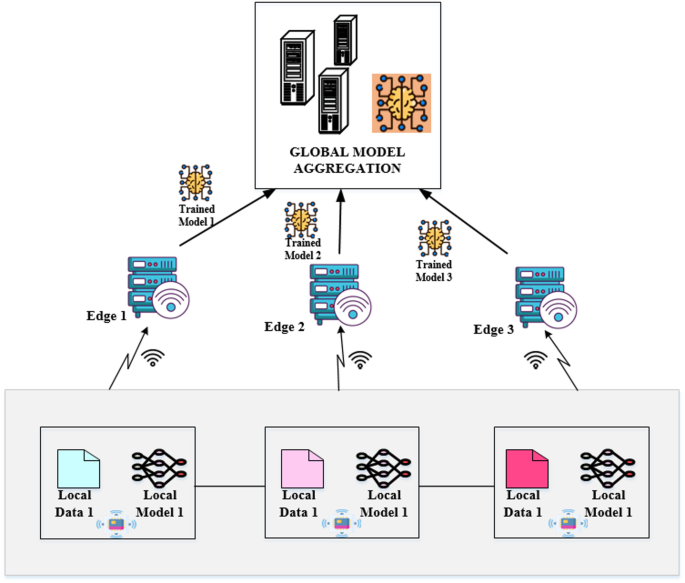
Workflow of federated learning.
Global model aggregation
Finally, after training the local models, the edge models need to aggregate those models towards forming a single global model, which is typically performed by the central server. The workflow of model aggregation is shown in Fig. 7.
Federated aggregation: The global server aggregates the model updates that come from each edge node by using a process called Federated Averaging, or FedAvg. It combines the model parameters (weights or gradients) coming from each of the edge nodes into a single unified model. This process can be represented mathematically as Eq. (9).
$$\:{w}_{global}=\frac{1}{N}\sum\:_{i=1}^{N}{w}_{i}$$
(9)
where, \(\:{w}_{global}\) denotes the aggregated global weight, \(\:{w}_{i}\) represents the weight from the \(\:{i}^{th}\) local model, \(\:N\) indicate the number of edge nodes. Because of non-synchronous device performance, straggler nodes – nodes that do not respond within a 30-s window, will not be included in the current round to prevent bottlenecks during training. Additionally, in order to reduce communication and synchronization overhead due to frequent updates being transmitted, model updates have been quantized, and devices are allowed to communicate every 5 local epoch instead of after each epoch. This reduces the bandwidth usage and increases the usable resource lifetime of edge devices, which is crucial in disaster-prone scenarios when deployed to the real world.
Fig. 7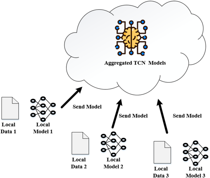
The aggregated model incorporates the knowledge learned from each disaster-specific dataset, making it robust across multiple disaster types. This enables the model now to predict broader sets of information, thus upgrading its ability toward predicting different forms of disasters and catastrophes, such as earthquakes, floods, and tsunamis.
Blockchain integration in federated learning for disaster prediction: working mechanism
The blockchain component of the mTCN-FChain framework is fundamental to securing federated learning operations by providing encrypted update transmission, tamper-proof validations, traceability, and resilient fault tolerance. For securing model updates sent from edge nodes, symmetric encryption using the AES-256 algorithm is utilized. Each model update is encrypted individually, instead of encrypting all updates in a single batch, before being sent to the blockchain so that confidentiality can be ensured for any gradient or weight vector shared from the local mTCN models.
Let \(\:M\in\:{\mathbb{R}}^{n}\) be the model update vector of an edge node, with nnn being the number of learnable parameters. The encrypted version \(\:C\) is represented as Eq. (10).
$$\:C={AES}_{K}\left(M\right)$$
(10)
where \(\:{AES}_{K}\) is the AES encryption function with a 256-bit key \(\:K\). The size of each update vector prior to encryption is between 320 KB and 512 KB based on the depth of the local mTCN model, whereas the encrypted output has an almost negligible overhead (~ 3–5%) attributed to AES block padding. The updates are pushed to the blockchain ledger every 5 local epochs, which coincides with the federated communication round interval to limit bandwidth consumption and power expenditure on resource-constrained edge devices.
Digital signatures are created with the ECDSA algorithm (Elliptic Curve Digital Signature Algorithm) using 256-bit keys. Let \(\:S\) be the digital signature of an update \(\:M\) created with the private key \(\:{K}_{priv}\), given in Eq. (11).
$$\:S={ECDSA}_{{K}_{priv}}\left(H\left(M\right)\right)$$
(11)
where \(\:H\left(M\right)\) represents the SHA-256 hash of the model update. After getting to the central aggregator, the signature \(\:S\) is verified with the sender public key \(\:{K}_{pub}\) to verify the source and integrity of the update. If the verification does not pass, the update is rejected and set to audit status. All verified updates are tracked on a permissioned blockchain based on Hyperledger Fabric. The ledger has nearly 1000 TPS of transaction throughput and utilizes a Proof-of-Stake (PoS) consensus with a ten second block time and one-megabyte block size limit. Each update stored includes a timestamp, node ID, update type (flood, earthquake, and tsunami) and cryptographic metadata. This immutable log provides complete traceability of contributions and allows for forensic analysis in real-time.
The framework is resistant to various types of attacks, e.g. tampering, model poisoning and spoofing. Hashed updates are automatically rejected at verification stage through hash mismatch. Attackers found to frequently fail in validating their gradients across rounds are blacklisted such that each malicious node trying to inject adversarial gradients is temporarily blocked from participating in the aggregation. In case of node compromise, the system can simply reinitialize the local model with the most recent global model and re-verify through a quorum of trusted validators before being allowed back into the network. This design guarantees the data Privacy, provenance and system robustness with reduced communication overhead. Security and integrity of disaster prediction as maintained within the federated environment are jointly secured by encryptions, digital signatures, as well as integrity backed by ledgers, coupled with traceability. The technical design of the system has been abided by most recent developments of safe federated learning29, making it accurate in case of high-risk real-time conditions.
Deployment and feedback
An updated model of global mTCN is deployed along with a feedback mechanism to effectively deploy real-time predictions of a disaster. The workflow of deployment and feedback is shown in Fig. 8.
Fig. 8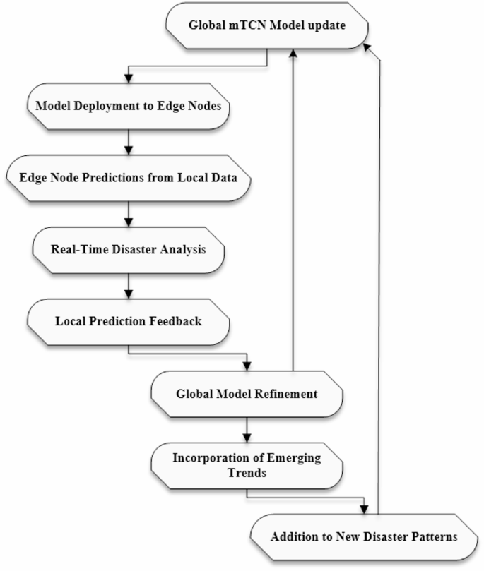
Flowchart of deployment and feedback.
Model deployment
Once the global mTCN model is updated through aggregation of the local model parameters, it gets deployed on all participating edge nodes. This enables every node to receive the most recent and updated version of the model for a real-time accurate prediction in a disaster situation. Disasters such as floods or earthquakes can be evaluated according to the latest known information. This allows the system to adapt to changing conditions and growing data sources.
Feedback loop
The feedback loop is critical for the continuous improvement and adaptability of the disaster prediction system. It has two main components:
Continuous learning
Once the global model has been deployed, each edge node generates predictions from real-time data. These predictions are fed back into the system for analysis. Feedback from local predictions allows for an iterative refinement of the global model. Mathematically, this may be represented as following Eq. (12).
$$\:\varDelta\:w=\eta\:\cdot\:\left({y}_{actual}-{y}_{prediction}\right)\cdot\:x$$
(12)
where, \(\:\varDelta\:w\) represents the change in model weights, \(\:\eta\:\) is the learning rate, \(\:{y}_{actual}\) denotes the actual observed outcome, \(\:{y}_{prediction}\:\)is the predicted outcome, \(\:x\) represents input features.
Adaptability
The feedback loop thus ensures that the mTCN model evolves with time as the pattern of disasters change. For example, in the case of an emerging type of flood event or an increase in seismic activity within a region once stable, the model can evolve from new data input. More information from the constant monitoring and predicting processes will be used for further training, which can constantly adapt to newly emerging trends and anomalies. Overall, the dynamic framework should enhance disaster preparedness and response capabilities well. This dynamic framework enhances better outcomes under emergency situations.
Algorithm of mTCN-FChain for disaster prediction
Input: Multi-modal disaster datasets (earthquake, flood, tsunami).
Output: Global disaster prediction model with real-time deployment.
1. datasets ← collect_datasets([“earthquake”, “flood”, “tsunami”])
2. preprocessed_data ← preprocess(datasets).
3. edge_nodes ← initialize_edge_nodes().
4. for each node in edge_nodes:
5. local_data ← get_data(node).
6. local_model[node] ← train_TCN(local_data).
7. for each node in local_model:
8. updates ← get_model_updates(local_model[node])
9. encrypted_update[node] ← encrypt(updates).
10. blockchain ← initialize_blockchain().
11. for each node in encrypted_update:
12. if verify_signature(encrypted_update[node], node.key)
13. store_on_blockchain(encrypted_update[node], node.signature)
14. validated_updates ← blockchain.get_validated_updates()
15. global_model ← aggregate_updates(validated_updates)
16. for each node in edge_nodes
17. distribute_model(global_model, node)
18. for each node in edge_nodes
19. predictions[node] ← predict(global_model, node.test_data)
20. repeat process with new data for continual learning
Fig. 9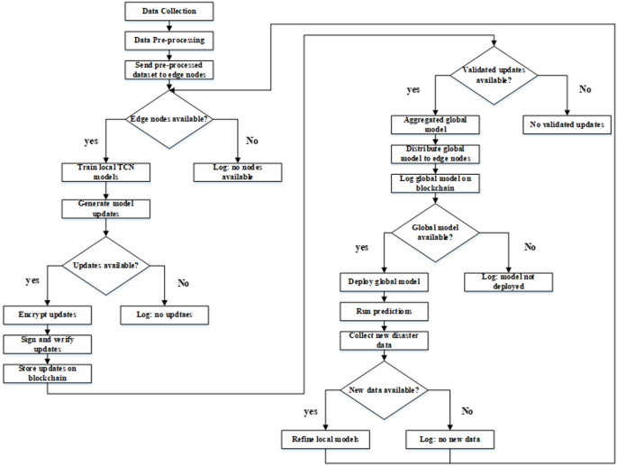
Flowchart of proposed method mTCN-FChain.
The mTCN-FChain framework is a novel framework that brings together Temporal Convolutional Networks, Federated Learning, and blockchain technology to enable disaster prediction in a secure, decentralized, and privacy-preserving manner. The framework makes use of a TCN model to model sequential data from multiple hazards; federated learning allows collaborative training by the edge devices without sharing or gathering data. The employment of blockchain ensures model trust and provenance. The complete operational flow of the proposed framework is given in Fig. 9.