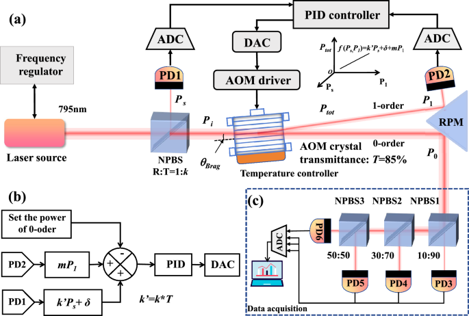
Our experimental setup is depicted in Fig. 1. The photoelectric control system is shown in Fig. 1a. A semiconductor laser (EYP-DFB-0795-00080-1500-BFW01-0005, TOPTICA) is used as the source. About 0.5 mW laser power is feed into the frequency regulator, which is used for locking the laser frequency to specific atomic transition line. The major beam power incidents into the NPBS with reflection to transmission ratio R:T=10:90. The transmitted beam goes into the AOM (model 3080-125, Gooch-Housego) at the Bragg angle, while the reflected beam is sampled by photodetector PD1 (PDA36A2, Thorlabs). The diffracted beams contains the 0th, 1st and higher-order beams. The 0th and 1st order beams exhibit insufficient spacing for direct measurement. To resolve this constraint, the optical path is extended. Subsequently, a right-angle prism mirror (RPM) is implemented to redirect the beams prior to measurement, while the higher-order beams are blocked. The 1st order beam is detected by photodetector PD2. As the high power of the 0th order beam can saturate a single photodetector, three NPBS and four photodetectors are used to split the beam and collect the beam powers accordingly, as shown in Fig. 1c. The detected voltages are digitized by an analog-to-digital converter (ADC) and subsequently processed through a data acquisition (DAQ) to estimate the results of power control. Since the diffraction efficiency of the AOM is sensitive to temperature fluctuations23,24,25, a TEC cooling plate and an NTC thermistor are used to control the temperature of the AOM housing to 23.02 ± 0.006 \(^{\circ }\)C. Photodetector PD1 measures the sampling beam power and characterizes the AOM incidence power. Photodetector PD2 measures the 1st order diffraction beam power and characterizes the temperature-sensitive term. In Fig. 1b, according to the set value of the 0th order beam power, a PID control algorithm is utilized to make the AOM driver adjusting the 1st order diffraction beam of the AOM.
Fig. 2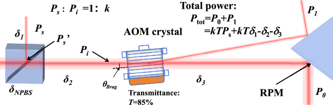
Schematic diagram showing the conservation law of the optical power distribution in the main optical path.
The control algorithm are designed based on the conservation law, which is revealed by a thorough analysis on the power distribution in optical path before and after the AOM, as shown in Fig. 2. First, the sampling beam power \(P_{s}\) and the power \(P_s^{‘}\) at the splitting interface of NPBS is given by
$$\begin{aligned} P_s = P_s^{‘} – \delta _1, \end{aligned}$$
(1)
where \(\delta _1\) is the attenuation caused by the NPBS and the air from the reflected point to PD1. The AOM incidence power \(P_{i}\) is given by
$$\begin{aligned} P_i = kP_s’ – \delta _2, \end{aligned}$$
(2)
where \(k\) \(\approx\)10 is the transmission to reflection ratio of NPBS, and \(\delta _2\) is the attenuation in between the splitting interface of NPBS and the incidence point of AOM. The total output power \(P_{tot}\) of the AOM can be given by
$$\begin{aligned} P_{tot} = T P_i – \delta _3, \end{aligned}$$
(3)
where \(T\) \(\approx\)85\(\%\) is the transmittance of the AOM crystal and \(\delta _3\) is the attenuation of incidence beam in the acousto-optic crystal and in the air. According to Eqs. (1)–(3), the total power at the measured position can be obtained
$$\begin{aligned} \begin{aligned} P_{tot}&= P_0 + P_1 \\ &= k T P_s + k T \delta _1 – \delta _2 – \delta _3 \\ &= k’ P_s + \delta , \end{aligned} \end{aligned}$$
(4)
where \(k’\)=kT. After establishing stable optical paths and components, the total attenuation will stay constant. We therefore define the composite attenuation constant as: \(\delta = k T \delta _1-\delta _2-\delta _3\). Since the diffraction efficiency in this experiment remains extremely low (\(), the power of higher order beams can be safely neglected in this case.
During experiments, we found the transmission of the AOM crystal increases with the temperature. To test the AOM’s temperature dependence, we turned off the frequency regulator and maintain a fixed driving current of laser source to ensure a constant beam power incident on the AOM. By turning off the AOM driver, we set the diffraction efficiency to zero and then adjust the housing temperature of the AOM, the transmission beam power versus the temperature is plotted in Fig. 3. It can be seen that the change of the transmission beam power with temperature is approximately linear, with a slope rate of about 0.018 \(\hbox {mW}/^{\circ }\)C.
Fig. 3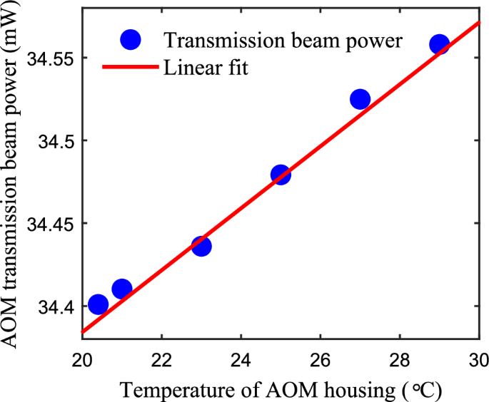
The transmission beam power measured as a function of the AOM housing temperature. The incident beam power on AOM is about 40 mW.
Fig. 4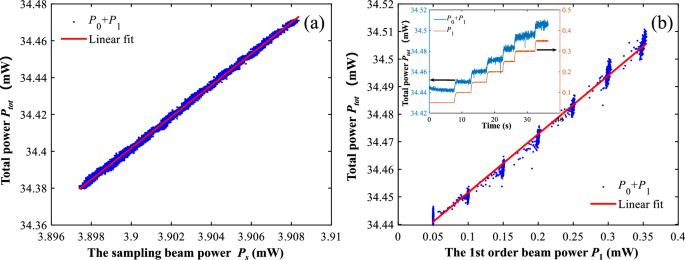
(a) The relationship between the total diffraction beam power \((P_0+P_1)\) and the sampling beam power \(P_s\). (b) The relationship between the total diffraction beam power \((P_0+P_1)\) and the 1st order beam power \(P_1\).
On the other hand, we noticed that the temperature of AOM crystal increases with the AOM driver output voltage23,24. Once the AOM is turned on, there should be an additional temperature-sensitive power fluctuation due to the heating effect of the nonzero AOM driver output. To address this issue quantitatively, we introduce a temperature-sensitive power term \(P_{T}\) into Eq. (4), which is now modified to be
$$\begin{aligned} P_{tot} = P_0 + P_1 = k’ P_s + \delta + P_T. \end{aligned}$$
(5)
When the diffraction efficiency is at a low level (\(), the temperature-sensitive power term is proportional to the AOM driver output voltage and thus the 1st order diffraction beam power, therefore Eq. (5) can be rewritten as
$$\begin{aligned} P_{tot} = P_0 +P_1 = k’ P_s + \delta + mP_1, \end{aligned}$$
(6)
where m is a unit-less coefficient of the temperature-sensitive power over the 1st order diffraction beam power \(P_1\).
To this end, we have derived the relationship between the 0th order diffraction beam power, the 1st order diffraction beam power and the sampling beam power from a theoretical perspective according to the power distribution analysis in Fig. 2. Furthermore, we have to prove this so-called conservation law experimentally. By tuning the driving current of the laser source, we measured the powers of the sampling beam, the 1st order diffraction beam and the 0th order diffraction beam with the photodetectors PD1, PD2 and PD3-PD6, respectively. The total power \(P_{tot}\) changes with the sampling beam power \(P_s\) and the 1st order diffraction beam power \(P_1\) approximately linearly, as shown in Fig. 4a,b, respectively. This proves the relationship in Eq. (6) is correct and gives us the values of coefficients \(k’=8.5301\), \(m=0.208\) and the value of constant attenuation \(\delta =1.1345\) mW through linear fittings.
Since all the power terms fluctuate with time, we can rewrite Eq. (6) as
$$\begin{aligned} P_0(t) = k’ P_s(t) + (m-1) P_1(t) +\delta . \end{aligned}$$
(7)
As m is smaller than one, the second term in Eq. (7) is actually negative. In order to keep the application beam power \(P_0(t)\) stable over time, we need to keep the difference between the total power \(P_{tot}\) given by Eq. (6) and the 1st order diffraction beam power \(P_1\) dynamically constant. This is done by the PID controller. It takes the power of the sampling beam and the 1st order beam (in Fig. 1a) as inputs, and outputs a calibrated AOM driver control voltage to adjust the diffraction beam power. The control voltage of AOM driver is calibrated using an algorithm depicted in Fig. 1b. The basic idea is to adjust the power of the 1st order beam in real time to follow the power of the sampling beam dynamically, as described by Eq. (7).
Fig. 5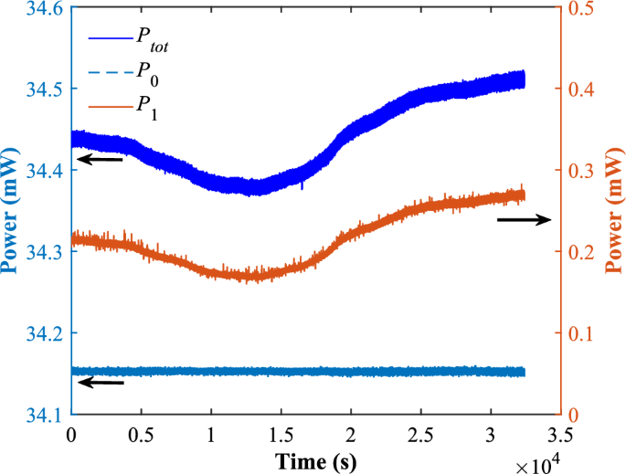
Temporal fluctuations of the total power \(P_{tot}\), the 1st order beam power \(P_1\) and the 0th order beam power \(P_0\) during the period of 9 h.