
For this study, we run CCAM at 12.5 km horizontal resolution (CCAM-12.5) and at 100 km horizontal resolution (CCAM-100). Both CCAM configurations are forced using spectral nudging for winds, air temperature and surface pressure from the fifth generation of the European Centre for Medium-Range Weather Forecasts atmospheric reanalysis (ERA527) over the 1980 to 2020 period. The two CCAM simulations have similar large scale features that come from nudging to ERA5 but differ in how they represent synoptic weather. These two simulations produce significantly different rainfall, particularly in the regions with strong orography and high mean rainfall (Fig. 1). The large difference between the two simulations shows the challenge ML must overcome to downscale CCAM-100 to the resolution of CCAM-12.5. For example, the mean climatological hourly rainfall of CCAM-12.5 is about 5x the CCAM-100 values. The scaling increases further as one compares the extreme hourly rainfall with CCAM-12.5, 5x greater at 90th percentile and 10x greater at the 99th percentile than CCAM-100 (Figs. 2 and 3). The ML downscaling of hourly rainfall must correct the mean, add spatial variability and enhance extremes to emulate the behaviour of the CCAM-12.5 (Figs. 1 and 2). In the following discussion, we first demonstrate a super resolution ML model can accurately downscale hourly rainfall from the coarsen CCAM-12.5 at 100 km resolution to the CCAM-12.5 values (target data). We call this ML downscaling model, MLPerfect. We then apply the MLPerfect to the CCAM-100 to see how well it can reproduce the CCAM-12.5 values. The downscaled rainfall lacks the variability present in CCAM-12.5 simulation, which motivates us to try another ML model. Finally, we train a super resolution ML to downscale the CCAM-100 values to CCAM12.5 and we call this downscaling model as MLImperfect.
Applicability of super-resolution ML approach to precipitation downscaling
First, we assess the ML models’ ability to predict the climatology of hourly precipitation for the test period (2012–2020), which we call the target data in Fig. 1a,c,i. The MLPerfect with coarsen CCAM-12.5 input captures well the target data (Fig. 1a,b). The MLImperfect with CCAM-100 as input also captures well the climatological rain as shown in Papua New Guinea (PNG) and southeast Australia (SEA) (Fig. 1h,n). Both models represent the fine-scale spatial structure of the climatology well, even when zoomed in on complex orographic regions like PNG and SEA compared to the target. The MLPerfect model better predicts the intensity of the fine-scale spatial pattern of the target data than the MLImperfect model (compare Fig. 1c–f,h,i–l,n). This is because MLPerfect only needs to learn the mapping between the perfectly aligned input and target (Fig. 1c vs. e,i vs. k), and the coarsened input partly preserves the fine-scale spatial pattern compared to the low resolution CCAM-100 simulation (compare Fig. 1e–d,k–j). The MLImperfect has more difficult task because it must learn the mapping from input to the target, which includes learning the spatial inconsistencies (compare Fig. 1d,c).
For comparison, the CCAM-100 simulation was used as input to the MLPerfect model (Fig. 1g,m). The resulting prediction fails to capture the spatial structure of climatology in the PNG and SEA regions (see Fig. 1g,m). Further, the prediction has high average rainfall over the southwestern parts of PNG instead in the central PNG region and creates a spatial mismatch of high average rainfall regions in the SEA domain as well compared to the target (compare Fig. 1c vs. g,i vs. m). This is because MLPerfect seems to be learned the mapping between coarse input and target, which is sharpening and increasing the rainfall values with fine-scale spatial structure around the regions of moderate precipitation values, for example, the central PNG region (see Fig. 1e,f) and northeast parts of SEA domain (Fig. 1k,l). Hence, MLPerfect with CCAM-100 simulation as input produces a high precipitation average in the southwest PNG region where the high rainfall climatology is seen in the CCAM-100 km simulation (Fig. 1d,g). This is also the same for the SEA domain; MLPrefect sharpened and increased the rainfall average around the high average precipitation region of the CCAM-100 km simulation (Fig. 1j,m). The power spectral density (PSD; calculated using the 2-dimensional Fast Fourier Transform as mentioned in Reddy et al. (2023)) of climatology shows that the MLPerfect with CCAM-100 km input underestimates the PSD at mid-range wavelengths compared to the target PSD (Fig. 1o). These results highlight the limitation of applying MLPerfect to input from a coarse resolution CCAM simulation making MLPerfect unsuitable for climate downscaling. In contrast, MLImperfect with the same low-resolution CCAM-100 input can reproduce the fine-scale spatial pattern of precipitation climatology of the target and appears to successfully downscale climatological rainfall (Fig. 1c vs. h).
Fig. 1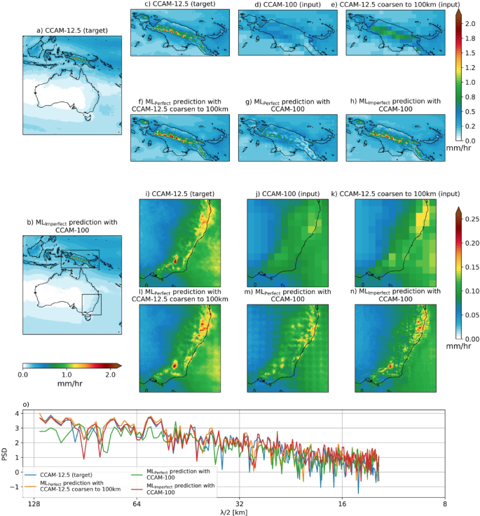
Climatology of hourly precipitation (mm/h) of CCAM 12.5 km target (a) and MLImperfect model predictions (b) over the study region during the test period. The top panels (c–h) show climatology over zoomed-in region of Papua New Guinea (PNG). Panel (c) shows CCAM-12.5 km target, (d) CCAM-100 km input, (e) CCAM-12.5 km coarsen to 100 km input, (f) MLPerfect model prediction with 12.5 km coarsen 100 km input, (g) MLPerfect model with CCAM 100 km input, and (h) MLImperfect model prediction climatology over the PNG region, respectively. Similar to top panel, middle panel (i–n) shows the climatology over the southeast Australia region (SEA). The line plot in the bottom panel (o) shows the power spectral density (shown only for mid-range and short wavelengths) of the climatology across the entire domain for different considered model predictions and the target. Maps are drawn using the Python Cartopy package (v0.24.1).
Figure 2 shows the 95th percentile maps of hourly precipitation of the CCAM 12.5 km target, for MLPerfect with coarsen CCAM-12.5 to 100 km input, MLPerfect with CCAM-100 input and MLImperfect with CCAM-100 input. Similar to the climatology results, MLPerfect with coarsen CCAM-12.5 input reproduces the fine-scale spatial pattern of extremes (95th percentile) well in the complex orographic regions of PNG (Fig. 2c,f) and SEA (Fig. 2i,l). However, MLPerfect with CCAM-100 input is not able to get the fine-scale spatial pattern of extremes and has spatial inconsistencies similar to the climatology as mentioned above (Fig. 2g vs. c,m vs. i). Whereas MLImperfect can reproduce the fine-scale spatial structure of extremes but underestimates the magnitude (Fig. 2h vs. c,n vs. i).
Fig. 2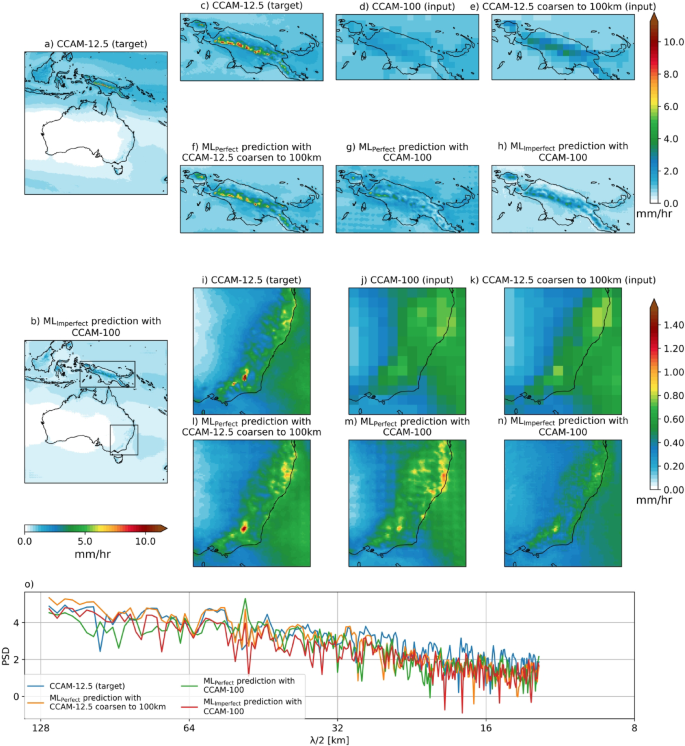
Same as Fig. 1 but for the 95th percentile of the hourly precipitation during the test period. Maps are drawn using the Python Cartopy package (v0.24.1).
We evaluate the ML performance by examining the relationship between climatology and extremes (90th, 95th, and 99th percentiles) by plotting the climatological mean value versus the corresponding extreme value (Fig. 3). The relationship allows one to assess the ML models without focusing on an exact grid point comparison, which is flawed because of chaotic weather processes. A comparison of the CCAM-12.5 simulated relationship to the CCAM-100 simulation shows the low resolution substantially underestimates both the climatological extreme rainfall. CCAM-100 is a poor reflection of the CCAM-12.5. MLPerfect with CCAM-12.5 coarsen input reproduces the mean and extreme relationship of the target for the 90th and 95th percentiles but underpredicts the 99th percentile values. For the 99th percentile, MLPerfect underestimates the relationship between the mean rainfall and the extreme value with an underprediction of the extreme values. MLPerfect with CCAM-100 input poorly predicts the mean and extreme relationship by underestimating both the mean and extreme values. MLImperfect with CCAM-100 input slightly underestimates the extreme values in the mean versus extreme relationship at the 90th percentile compared to the target (Fig. 3a). The MLImperfect under prediction of the extremes become more evident for rainfall extremes above the 90th percentile with an underprediction by 2.5x and 6x for the 95th and 99th percentile, respectively (Fig. 3b,c).
Fig. 3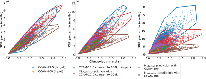
Scatter plot comparison of mean versus extreme relationship (climatology versus 90th percentile (a), versus 95th percentile (b), and versus 99th percentile (c), respectively) among the CCAM-12.5 km target (blue), CCAM-100 km simulation (orange), CCAM-12.5 coarsen to 100 km input (green), MLPerfect model predictions with CCAM-12.5 coarsen to 100 km input (red), MLPerfect model with CCAM-100 km input (purple), and MLImperfect model predictions with CCAM-100 km input (brown).
ML model sensitivity investigation – explainable ML experiments
To understand the behaviour of the ML model for precipitation downscaling we performed several input perturbation sensitivity experiments. First, we present the results of the MLPerfect and MLImperfect predictions when the input is zero precipitation values at all grid points with the additional orography input (shown in Fig. 4). The MLPerfect model predicts zero precipitation everywhere except in PNG high altitude regions with very small values 4a). However, MLImperfect with zero rainfall input predicts zero precipitation in the non-tropical regions of the domain and precipitation values of around 0.2–0.9 mm/h in the high-altitude tropical regions of the domain, particularly the elevated parts of the PNG region (Fig. 4b). The MLImperfect rainfall prediction is converting the orographic input into precipitation outputs (accounts up to 40% of the mean value). To further understand the effects of the orography signal on the ML-predicted rainfall, we conducted the input perturbation experiments at the three selected locations in the domain. Three locations are chosen in the high-altitude PNG region, SEA land region, and the Southern Ocean (SO) region, respectively (see Fig. 5a). Now, the input perturbation with 0.5 mm/h is performed at these locations, with the rest of the grid points are zeros. With this point perturbation at all three locations, the MLPerfect predictions are concentrated at and near the perturbation point with very small precipitation (5b–d). However, MLImperfect predicts precipitation around 0.5–0.9 mm/h over the high-altitude tropical regions of the domain irrespective of perturbations at the three selected locations (Fig. 5e–g). Further, we performed the input perturbations with 1 mm/h at three selected locations and the results are similar to the 0.5 mm/h input perturbation (Fig. S3). MLImperfect predicts precipitation at the high-altitude regions of the domain no matter the input, because it is getting the signal from the additional orography input. MLImperfect is utilising the topography in the model to map CCAM-100 to the CCAM-12.5 simulation by adding rainfall where it consistently underestimates rainfall resolution enhancements.
Fig. 4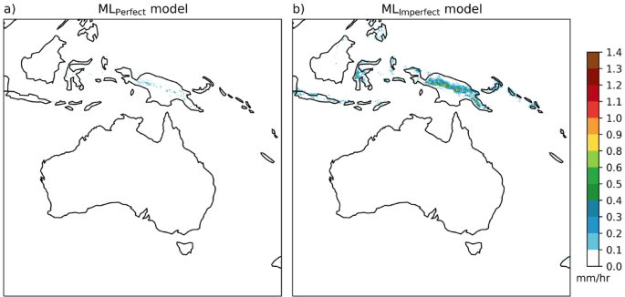
MLPerfect (a) and MLImperfect (b) model output precipitation (at 12.5 km) when provided zero coarse precipitation input (at 100 km) on all grid points and the additional orography input unchanged. Maps are drawn using the Python Cartopy package (v0.24.1).
Fig. 5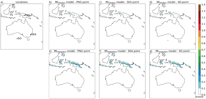
MLPerfect and MLImperfect model output precipitation (at 12.5 km) when provided zero coarse precipitation input (at 100 km) on all grid points except a small precipitation perturbation of 0.5 mm/h at the three selected points (one in Papua New Gunia (PNG), second in South East Australia (SEA), and the third in Southern Ocean (SO) as shown in (a)), each point perturbation at a time and the orography input is unchanged. MLPerfect and MLImperfect model output precipitation when perturbed at the PNG point with orography unchanged are shown in (b) and (e), respectively. The MLPerfect and MLImperfect model outputs when perturbed at SEA and SO points are shown in (c), (f) and (d), (g), respectively. Maps are drawn using the Python Cartopy package (v0.24.1).
Here, we present the results of ML prediction for various input perturbations to understand and explain the behaviour of super-resolution ML models in precipitation downscaling. Figure 6 shows the model response diagnostics (maximum response and number of responses) of MLPerfect and MLImperfect when perturbed with 0.5 and 1 mm/h. MLPerfect model amplified the input perturbation across all the regions of the domain, i.e., when perturbed with 0.5 mm/h the maximum response ranges from around 2–7.5 times the perturbation and with 1 mm/h the maximum response ranges from 2 to 10 times the perturbation (Fig. 6a,b). Further tested with perturbations 5 and 10 mm/h, which resulted in maximum response ranges around 2.38–5 and 3–5 times the perturbation, respectively (Fig. S4a,b). The MLPerfect shows a non-linear response with the scaling factor changing with the magnitude of the input perturbations. Consistent with sharpening up the coarse rainfall input, the maximum response is greater than 1. Given the 8x downscaling in the latitude and longitude, if the input rain was concentrated in just one grid cell of the fine resolution grid, the maximum response would be 64x the input value. The maximum response of the MLPerfect varies across the domain such as some parts of the tropical land regions have the highest maximum response values, and some parts of the orographic regions over Australia have the lowest maximum response values compared to the other regions of the domain. This is because in the orographic regions the MLPerfect model responded at many grid points, which probably means that the model is spreading out the input precipitation over neighbouring grid points with not spiking it too much at or next to the perturbed point (Fig. 6e,f).
Further, we have looked at the impact distance, to see how far the model response extends from the input perturbation. Results show that the maximum value of impact distance at all grid points is around 500 km (not shown), which is very close to the input perturbation grid point. This suggests that the MLPerfect model did not learn any spatially spurious relationships. This is because the ML models are fully convolutional, where the filters/kernels mostly learn the spatially constrained information over a finite space. Similar to the MLPerfect model, MLImperfect model extrapolated the input perturbations across the domain with maximum values over the PNG region. Perturbing with 0.5 mm/h the MLImperfect model responses range from around 2–6 times the perturbation and with 1 mm/h perturbation the model responses range from around 1.3–3.4 times the perturbation. The MLImperfect model responses are not varying much over the domain except in the PNG region, where the large variations are seen (Fig. 6c,d). MLImperfect fails to produce much scaling up of the input for the rest of the domain. MLImperfect does much less amplification of the input rainfall than the MLPerfect. There is strong non-linearity in the number of maximum responses in the MLImperfect in Australia. Doubling the input rainfall leads to more than 4x more responses. Consistent with the reduced amplification of the rainfall input, the MLImperfect spread the input rainfall of 1 mm/h over an order of magnitude more fine-resolution grid points than MLPerfect. The MLPerfect and MLImperfect behave very differently in both the maximum response and in the number of responses and how it changes in input value – one responding to the bias and one correcting missing features.
Fig. 6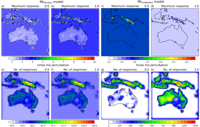
MLPerfect model response diagnostics (maximum response (a) and number of responses (e)) when perturbed with 0.5 mm/h input at a particular grid point and made rest all grid points as zero; and in the same way iteratively executed at all grid points. MLPerfect model response diagnostics when perturbed with 1 mm/h input are shown in subplots (b; maximum response) and (f; number of responses). MLImperfect model response diagnostics when perturbed with 0.5 and 1 mm/h input are shown in subplots (c; maximum response), (g; number of responses) and (d; maximum response), (h; number of responses), respectively. For more details about model response diagnostics refer to data and methods section. Maps are drawn using the Python Cartopy package (v0.24.1).