Discrete wavelet packet
Wavelet Packet Transform (WPT) is a sophisticated signal processing technology that extends traditional wavelet conversion by allowing more flexible decomposition of signals into distinct frequency bands. Unlike the discrete wavelet transform, which divides signals only into approximation and detail coefficients, WPT decomposes both low-frequency (approximation) and high-frequency (detail) components. It utilizes a series of low-pass and high-pass filters to split the signal across multiple levels, with each level providing a set of coefficients that represent signal characteristics in various frequency bands. This enables comprehensive analysis of transient events, such as faults in transmission lines. The coefficients obtained from WPT are used as input features for neural network models. Due to its ability to capture transient behavior and local signal variations, WPT is particularly effective for fault diagnosis. It supports signal analysis with varying levels of accuracy, which is essential for identifying faults occurring over different time scales. Additionally, filtering development helps eliminate noise and improves the quality of features used to train ML models. Wavelet decomposition is generalized by the WPT approach, which provides more possibilities for signal analysis. WPT eliminates high-frequency and low-frequency signal components using low- and high-pass filters. Splitting the filtered signals is the next step in processing, performed as often as needed. The original signal processed by successive pairings of high-pass filters (HPFs) and low-pass filters (LPFs) is represented by f(t) in Fig. 3, which shows a signal decomposition employing WPT.
Fig. 3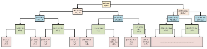
Discrete WPT-based analysis.
The low-scale high-frequency components in each pair are called details (D1), while the high-scale low-frequency components are called approximations (A1). According to Nyquist’s rule, every second data point is eliminated after each filtering stage. This procedure, called down-sampling, avoids redundant data. The signal’s CWT can be calculated by multiplying the sum of the signal’s f(t) over all time by a scaled and shifted version of the mother wavelet ψ(t), which is expressed as:
$$\:{{\uppsi\:}}_{x,y}\left(t\right)=\frac{1}{\sqrt{x}}{\uppsi\:}\left(\frac{t-y}{x}\right)$$
(1)
where the time-shifting and time-scaling parameters are denoted by y and x. Consequently, the CWT is provided by:
$$\:CWT\:\left(x,\:y\right)={\int\:}_{-\infty}^{+ \infty}f\left(t\right).{{\uppsi\:}}_{y,x}^{*}\left(t\right).dt$$
(2)
where the complex conjugate is indicated by “*” A discrete signal’s WPT can be expressed as follows:
$$\:WPT\:\left(m,\:n\right)=\frac{1}{\sqrt{{a}_{0}^{m}}}{\sum\:}_{K}f\left(k\right){{\uppsi\:}}^{*}\left(\frac{n-k{a}_{0}^{m}}{{a}_{0}^{m}}\right)$$
(3)
In this instance, \(\:{a}_{0}^{m}\) and \(\:k{a}_{0}^{m}\) are used in place of the parameters x and y in Eqs. (1) and (2), respectively. The db10 wavelet was found to depict fault patterns after thorough analysis best. As indicated in Table 1, the sampled voltage and current signals were divided into four levels using the db10 wavelet to provide approximation coefficients across seven nodes at various frequency ranges.
Table 1 The four-level nodes suggested in a variable frequency range.
Consider a single line-to-ground fault in circuit 1 at 20 ms to extract the voltage and current signals of the two circuits under fault conditions. As depicted in Fig. 4, an AG fault in circuit 1 simultaneously causes the phase A current to increase while the other phases’ currents stay constant. Two networks have been employed in this work: one for FL and the other for FD and directional identification of the fault section.
Fig. 4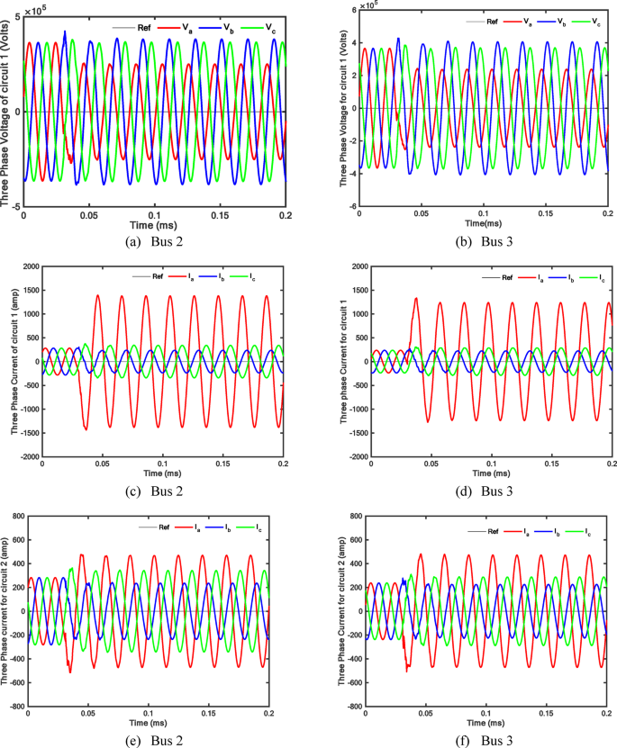
Double-circuit line 3Ph voltage and current signals during AG fault in circuit 1 of the selected system.
Nine indices, representing the WPT approximation coefficients for voltage and current samples from circuits 1 and 2 at both ends in each bus, are employed as inputs for two networks. These indices are given as follows:
$$\:{X}_{1}=\left[{A}_{Isa1\:}{A}_{Isb1\:\:}{A}_{Isc1\:\:}{A}_{Isa2\:}{A}_{Isb2\:\:}{A}_{Isc2\:\:}{A}_{vsa\:}{A}_{vsb\:}{A}_{vsc\:}\right]$$
(4)
$$\:{\:X}_{2}=\left[{A}_{Ira1\:}{A}_{Irb1\:\:}{A}_{Irc1\:\:}{A}_{Ira2\:}{A}_{Irb2\:\:}{A}_{Irc2\:\:}{A}_{vra\:}{A}_{vrb\:}{A}_{vrc\:}\right]$$
(5)
The foundation of each circuit’s FD module is monitoring variations in the WPT approximation coefficients for the three voltage and current samples in relation to their values during abnormal operation. Two fundamental ideas form the basis of the FSI module. First, the FSI module’s first output, which contains three outputs corresponding to Sects. 1, 2, and 3, serves as the foundation for the fault section concept. If no fault exists, the output is zero; if a section is faulty, it is one.
$$\:Y1=\left[{S}_{1\:}{S}_{2\:}{S}_{3\:}\right]$$
(6)
Second, extracting transient features from the approximation coefficients of the aerial mode currents (A4_ir) and (A4_vr) voltages is necessary for the directional identification of the fault section. The power over two cycles is added together to determine the aerial transient power index, 2N denotes the total number of samples in a window, and n denotes the sliding window sample order, as follows:
$$\:{P}_{A4}\left(k\right)=sign\left[{\sum\:}_{n=k-2N+1}^{k}\left|{D}_{4\_vr}*{D}_{4\_ir}\right|\right]$$
(7)
Thus, PA4 (k) specifies the transient direction of power depending on its polarity. The fault direction is determined by the polarity of this transient power index; a negative value indicates a forward fault, and a positive value indicates a reverse fault.
Fault location algorithm
The FL module uses the algorithm described in91 to estimate the FL. The single-line diagram for a single segment of the simulated DCTL is shown in Fig. 5. The lump parameter equivalent circuit during a fault is depicted in Fig. 6.
Fig. 5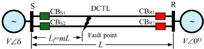
Single line diagram for one section of the investigated DCTL.
Fig. 6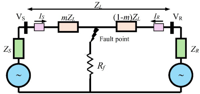
Lumped parameters equivalent circuit during fault.
The following formula is used to determine the 3Ph voltages at the fault point from both ends:
$${\left[ {{V_S}} \right]_{abc}} – {\left[ {{V_R}} \right]_{abc}}=m{\left[ {{Z_L}} \right]_{abc}}{\left[ {{I_S}} \right]_{abc}} – \left( {1 – m} \right){\left[ {{Z_L}} \right]_{abc}}{\left[ {{I_R}} \right]_{abc}}$$
(8)
where m is the location of the fault per unit along the line. The overall line impedance is [ZL]abc. The three-phase currents and voltages at the transmitting and receiving ends are [Is]abc, [IR]abc, [Vs]abc and [VR]abc, respectively.
$${\left[ {\Delta V} \right]_{abc}}+{\left[ {{Z_L}} \right]_{abc}}{\left[ {{I_R}} \right]_{abc}}=m{\left[ {{Z_L}} \right]_{abc}}{\left[ {\Sigma I} \right]_{abc}}$$
(9)
where:
\(\begin{gathered} {\left[ {\Delta V} \right]_{abc}}={\left[ {{V_S}} \right]_{abc}} – {\left[ {{V_R}} \right]_{abc}}, \hfill \\ {\left[ {\Sigma I} \right]_{abc}}={\left[ {{I_S}} \right]_{abc}}+{\left[ {{I_R}} \right]_{abc}}. \hfill \\ \end{gathered}\)
One can write (8) using the symmetrical transformation as follows92 :
$${\left[ {\Delta V} \right]_{012}}+{\left[ {{Z_L}} \right]_{012}}{\left[ {{I_R}} \right]_{012}}=m{\left[ {{Z_L}} \right]_{012}}{\left[ {\Sigma I} \right]_{012}}$$
(10)
It is necessary to extend (10) to take into consideration the mutual coupling between the two parallel circuits to reduce estimation errors brought on by mutual coupling:
$$\begin{gathered} \left[ {\begin{array}{*{20}{c}} {{{\left( {{{\left[ {\Delta V} \right]}_{012}}} \right)}_{Cir1}}} \\ {{{\left( {{{\left[ {\Delta V} \right]}_{012}}} \right)}_{Cir2}}} \end{array}} \right]+\left[ {\begin{array}{*{20}{c}} {{{\left( {{{\left[ {{Z_L}} \right]}_{012}}} \right)}_{self}}}&{{{\left( {{{\left[ {{Z_L}} \right]}_{012}}} \right)}_{mutual}}} \\ {{{\left( {{{\left[ {{Z_L}} \right]}_{012}}} \right)}_{mutual}}}&{{{\left( {{{\left[ {{Z_L}} \right]}_{012}}} \right)}_{self}}} \end{array}} \right]\left[ {\begin{array}{*{20}{c}} {{{\left( {{{\left[ {{I_R}} \right]}_{012}}} \right)}_{Cir1}}} \\ {{{\left( {{{\left[ {{I_R}} \right]}_{012}}} \right)}_{Cir2}}} \end{array}} \right] \hfill \\ {\text{ }}=m\left[ {\begin{array}{*{20}{c}} {{{\left( {{{\left[ {{Z_L}} \right]}_{012}}} \right)}_{self}}}&{{{\left( {{{\left[ {{Z_L}} \right]}_{012}}} \right)}_{mutual}}} \\ {{{\left( {{{\left[ {{Z_L}} \right]}_{012}}} \right)}_{mutual}}}&{{{\left( {{{\left[ {{Z_L}} \right]}_{012}}} \right)}_{self}}} \end{array}} \right]\left[ {\begin{array}{*{20}{c}} {{{\left( {{{\left[ {\Sigma I} \right]}_{012}}} \right)}_{Cir1}}} \\ {{{\left( {{{\left[ {\Sigma I} \right]}_{012}}} \right)}_{Cir2}}} \end{array}} \right] \hfill \\ \end{gathered}$$
(11)
where, the self and mutual indices represent the self and mutual impedances between the circuits, with Cir1 and Cir2 denoting the first and second circuits. Using the positive sequence components, the formula for the first circuit becomes:
$$\begin{gathered} {\left( {\Delta {V_1}} \right)_{Cir1}}+{\left( {{Z_{L1}}} \right)_{self}}{\left( {{I_{R1}}} \right)_{Cir1}}+{\left( {{Z_{L1}}} \right)_{mutual}}{\left( {{I_{R1}}} \right)_{Cir2}} \hfill \\ {\text{ }}=m\left( {{{\left( {{Z_{L1}}} \right)}_{self}}{{\left( {\Sigma {I_1}} \right)}_{Cir1}}+{{\left( {{Z_{L1}}} \right)}_{mutual}}{{\left( {\Sigma {I_1}} \right)}_{Cir2}}} \right) \hfill \\ \end{gathered}$$
(12)
Then, (ΔV1)Cir1 can then be formulated as:
$$\begin{gathered} {\left( {\Delta {V_1}} \right)_{Cir1}}=m{\left( {{Z_{L1}}} \right)_{self}}{\left( {\Sigma {I_1}} \right)_{Cir1}} – {\left( {{Z_{L1}}} \right)_{self}}{\left( {{I_{R1}}} \right)_{Cir1}} \hfill \\ {\text{ }}+m{\left( {{Z_{L1}}} \right)_{mutual}}{\left( {\Sigma {I_1}} \right)_{Cir2}} – {\left( {{Z_{L1}}} \right)_{mutual}}{\left( {{I_{R1}}} \right)_{Cir2}} \hfill \\ \end{gathered}$$
(13)
Considering the phasor measurements at time t = t1, then (13) can be rewritten as,
$$\begin{gathered} {\left( {\Delta {V_1}\left( {{t_1}} \right)} \right)_{Cir1}}=m{\left( {{Z_{L1}}} \right)_{self}}{\left( {\Sigma {I_1}\left( {{t_1}} \right)} \right)_{Cir1}} – {\left( {{Z_{L1}}} \right)_{self}}{\left( {{I_{R1}}\left( {{t_1}} \right)} \right)_{Cir1}} \hfill \\ {\text{ }}+m{\left( {{Z_{L1}}} \right)_{mutual}}{\left( {\Sigma {I_1}\left( {{t_1}} \right)} \right)_{Cir2}} – {\left( {{Z_{L1}}} \right)_{mutual}}{\left( {{I_{R1}}\left( {{t_1}} \right)} \right)_{Cir2}} \hfill \\ \end{gathered}$$
(14)
By applying the above equation over four successive samples taken at constant time intervals Δt, four consecutive equations can be generated:
$$\left[ {\begin{array}{*{20}{c}} {{{\left( {\Delta {V_1}\left( {{t_4}} \right)} \right)}_{Cir1}}} \\ {{{\left( {\Delta {V_1}\left( {{t_3}} \right)} \right)}_{Cir1}}} \\ {{{\left( {\Delta {V_1}\left( {{t_2}} \right)} \right)}_{Cir1}}} \\ {{{\left( {\Delta {V_1}\left( {{t_1}} \right)} \right)}_{Cir1}}} \end{array}} \right]=\left[ {\begin{array}{*{20}{c}} {{{\left( {\Sigma {I_1}\left( {{t_4}} \right)} \right)}_{Cir1}}}&{{{\left( {{I_{R1}}\left( {{t_4}} \right)} \right)}_{Cir1}}}&{{{\left( {\Sigma {I_1}\left( {{t_4}} \right)} \right)}_{Cir2}}}&{{{\left( {{I_{R1}}\left( {{t_4}} \right)} \right)}_{Cir2}}} \\ {{{\left( {\Sigma {I_1}\left( {{t_3}} \right)} \right)}_{Cir1}}}&{{{\left( {{I_{R1}}\left( {{t_3}} \right)} \right)}_{Cir1}}}&{{{\left( {\Sigma {I_1}\left( {{t_3}} \right)} \right)}_{Cir2}}}&{{{\left( {{I_{R1}}\left( {{t_3}} \right)} \right)}_{Cir2}}} \\ {{{\left( {\Sigma {I_1}\left( {{t_2}} \right)} \right)}_{Cir1}}}&{{{\left( {{I_{R1}}\left( {{t_2}} \right)} \right)}_{Cir1}}}&{{{\left( {\Sigma {I_1}\left( {{t_2}} \right)} \right)}_{Cir2}}}&{{{\left( {{I_{R1}}\left( {{t_2}} \right)} \right)}_{Cir2}}} \\ {{{\left( {\Sigma {I_1}\left( {{t_1}} \right)} \right)}_{Cir1}}}&{{{\left( {{I_{R1}}\left( {{t_1}} \right)} \right)}_{Cir1}}}&{{{\left( {\Sigma {I_1}\left( {{t_1}} \right)} \right)}_{Cir2}}}&{{{\left( {{I_{R1}}\left( {{t_1}} \right)} \right)}_{Cir2}}} \end{array}} \right]\left[ {\begin{array}{*{20}{c}} {m{{\left( {{Z_{L1}}} \right)}_{self}}} \\ {{{\left( {{Z_{L1}}} \right)}_{self}}} \\ {m{{\left( {{Z_{L1}}} \right)}_{mutual}}} \\ {{{\left( {{Z_{L1}}} \right)}_{mutual}}} \end{array}} \right]$$
(15)
Equation (15) can subsequently be rewritten as:
$$\left[ {{V_n}} \right]=\left[ {{I_n}} \right]\left[ {\begin{array}{*{20}{c}} {m{{\left( {{Z_{L1}}} \right)}_{self}}} \\ {{{\left( {{Z_{L1}}} \right)}_{self}}} \\ {m{{\left( {{Z_{L1}}} \right)}_{mutual}}} \\ {{{\left( {{Z_{L1}}} \right)}_{mutual}}} \end{array}} \right]$$
(16)
The ratio between the unknowns (m(ZL1)self and (ZL1)self) should then be calculated by solving (16) instead of determining their exact values. The time required for computation is decreased because this ratio can be computed even with fewer equations. Equation (16) is solved as follows:
$$\left[ {\begin{array}{*{20}{c}} {m{{\left( {{Z_{L1}}} \right)}_{self}}} \\ {{{\left( {{Z_{L1}}} \right)}_{self}}} \\ {m{{\left( {{Z_{L1}}} \right)}_{mutual}}} \\ {{{\left( {{Z_{L1}}} \right)}_{mutual}}} \end{array}} \right]={\left[ {{I_n}} \right]^{ – 1}}\left[ {{V_n}} \right]$$
(17)
The local fault location Lf along line length L can then be calculated as follows:
$$\:{L}_{f}=m\times\:L=\left(\frac{m({{Z}_{L}}_{1}{)}_{self}}{({{Z}_{L}}_{1}{)}_{self}}\right)L$$
(18)
This algorithm’s output, m, is chosen to train the other network model, which provides the estimated FL output D.
$$\:Y2=\left[m\right]$$
(19)
Models of neural networks
In recent years, there has been an increasing dependence on advanced AI technologies to address complex tasks across various fields. The ability to automatically extract significant features from raw data, without widespread manual intervention, enhances the accuracy and scalability of fault diagnosis. The proven effectiveness of these AI approaches in modular studies corroborates their superiority over conventional methods, supporting their pivotal role in the development of modern fault diagnosis techniques. Three ML models (DL, CNNs, and RNNs) were employed for the fault diagnosis system, each carefully selected based on its unique strengths in handling different aspects of data. The selected ML models were trained and tested offline to ensure robust performance across various operational conditions. To achieve a highly generalized algorithm, a dataset was prepared, encompassing comprehensive variations in fault occurrences. Specifically, the dataset included 5,000 distinct fault scenarios, covering a range of fault distances from 0.1 to 1.0% in increments of 0.1%, and from 0.1 to 1% in increments of 0.1% for fault resistance scenarios and arcing faults. Additionally, the same fault cases were considered for changing the fault inception angle from 0 to 180°, along with corresponding changes to the fault distance and resistance. Furthermore, changing the boundary condition location was included.
Deep learning network architecture
The architecture of the proposed DNN for the fault diagnosis system is shown in Fig. 7. The input layer consists of 10 neurons accepting X1, X2, Y1, PA4, and Y2 formats, as derived in the fault features section. A complex-split mechanism is used to process these inputs effectively. The 1 st hidden layer is a fully connected dense layer with 8 neurons, using the hyperbolic tangent (tanh) activation function. This layer begins the feature extraction process by introducing non-linearity and transforming the input into a more abstract representation.
Fig. 7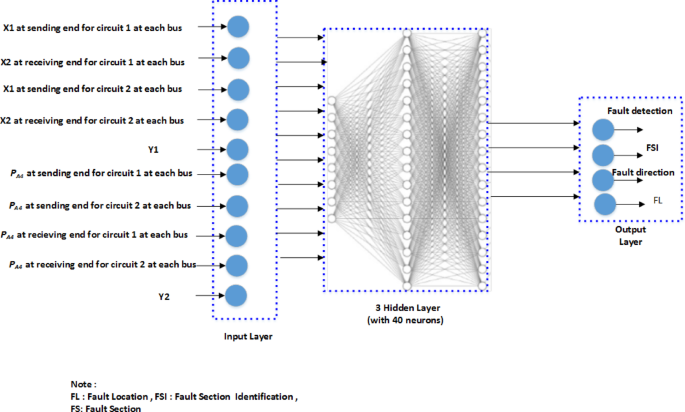
MLP model diagram: DL concept illustration.
The 2nd hidden layer, another fully connected layer, expanded to 16 neurons and uses tanh activation. With its deeper structure, it captures more complex patterns, enhancing the model’s ability to generalize. The 3rd hidden layer is a fully connected layer with 16 neurons, utilizing the rectified linear unit (ReLU) activation. ReLU helps mitigate the vanishing gradient problem, improves training efficiency, and promotes sparsity for better fault discrimination. The output layer is the final fully connected dense layer of the neural network, consisting of 4 neurons. It is responsible for producing the network’s output based on the learned representations from the previous layers. The three-output layer uses the sigmoid activation function, which maps the output to a probability range between 0 and 1, and the one-output layer uses ReLU activation. The training and testing of the DL model were utilized for developing a robust predictive model. 80% of the data set (4000 cases) was used for training, while the remaining 20% (1000 cases) was reserved for validation. The data partitioning was done randomly to ensure the model’s performance could be accurately assessed across a diverse range of data points, minimizing biases and ensuring reliability in real-world applications.
The DL model was implemented using the MATLAB Deep Learning Toolbox, which provides a comprehensive environment for designing, training, and validating deep learning models. This toolbox is well-suited for handling large datasets and complex model architectures. Training of the DL model was performed using the SGDM optimization algorithm, known for its efficiency in handling large datasets and complex models within the MATLAB Deep Learning Toolbox. The training process was structured to span a maximum of 100 epochs, with convergence typically achieved within just 20 epochs, totaling 7888 iterations. The initial learning rate was set at 0.01, with a learning rate reduction mechanism applied after each epoch. This adaptive learning rate strategy involves reducing the learning rate sequentially, which refines the adjustments made by the optimizer as training progresses. This method of dynamically adjusting the learning rate is critical for optimizing the training process and enhancing the model’s performance in fault detection tasks. A batch size of 64 was used, which is optimal for balancing the computational load and effective handling of the dataset size. The categorical cross-entropy loss function was employed, appropriate for the multi-class classification framework of our study.
Convolutional neural networks (CNNs)
CNNs are a class of deep learning models particularly effective for processing grid-like data, such as images or time-series signals. They consist of multiple layers, including convolutional layers that automatically learn spatial hierarchies of features. Although they can also be used to solve regression issues, CNNs, also known as ConvNets, are a specific ANN frequently employed for image processing and classification applications. When it comes to image, speech, or audio signal inputs, CNNs perform better. CNN comprises a fully connected feedforward neural network, a pooling part, and a convolutional (Conv) part. The central component, the convolutional section, has three important hyperparameters – the number of filters that determines the output’s depth, the filter or kernel’s stride that represents the distance it travels over the input matrix, and zero padding when the filters do not fit the input matrix. The sigmoid and ReLU activation is used to add non-linearity following each convolution operation. The pooling part then decreases the volume size. As depicted in Fig. 8, ConvNets’ primary component design is shown, where numbers are used as an example to demonstrate the convolution and pooling processes.
Fig. 8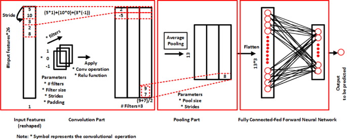
ConvNets’ primary component design (using numbers as an example to demonstrate convolution and pooling processes).
CNNs are well-suited for identifying patterns and features in spatial data, making them effective for analyzing the spatial characteristics of fault signals. They reduce the number of parameters through shared weights, which helps in generalizing the model and preventing overfitting.
Recurrent neural networks (RNNs)
RNNs are designed for sequential data, allowing for the processing of data where temporal contexts is important. They maintain a memory of previous inputs, making them suitable for time-series data. An RNN model’s architecture is depicted in Fig. 9. The output variable in the RNN is called yt., while the input variable at time step t is called xt. The hidden state st, which is determined using the current input xt and the prior hidden state st−1 from the previous time step, is the key component. The current input xt and the preceding hidden state st-1 determine the hidden state. The current hidden state, st, determines the output, yt.
Fig. 9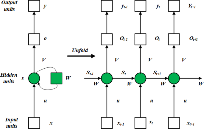
A simple construction of the RNN.
Because of the recursive link between the hidden states, the RNN can efficiently handle sequential data by retaining a “memory” of prior inputs. The following is an expression for an RNN’s mathematical model:
$$\:{s}^{t}=f\left(U\cdot\:{x}^{t}+b\right)$$
(20)
$$\:{o}^{t}=\left(V \cdot\:{s}^{t}+c\right)$$
(21)
$$\:{y}^{t}=g\left({o}^{t}\right)$$
(22)
The RNN model consists of weight matrices that define the connections between the layers, where the weight matrix between the input and hidden layers is \(U \in R^{lx \times ls}\), the weight matrix between the hidden layers is \(W \in R^{ls \times ls}\), and the weight matrix between the output and the hidden layers is \(V \in R^{lo \times ls}\). These weight matrices’ (U, W, V) values remain constant during the various time steps. The number of neurons in the input, hidden, and output layers is denoted by the variables x, ls, and lo, respectively. The RNN’s “memory” is the hidden state st at t, determined by the previous hidden state st−1 and the current input xt. The activation functions f = tanh and g = sigmoid, ReLU for the hidden layer and output layer, respectively, are used to compute the output ot that relies on the current hidden state st only. The bias vectors utilized in the computations are denoted by the parameters b and c. RNNs are adept at capturing temporal relationships in data, which is critical for analyzing time-varying signals during fault events. RNNs can handle variable-length input sequences, making them flexible for different fault scenarios and signal lengths. The ability to remember previous states allows RNNs to understand the context of faults over time, which enhances diagnostic accuracy.
Algorithm outline
Concerning the selected system shown in Fig. 2, the proposed fault diagnosis is dependent on WPT. The scenarios of fault detection, section, the direction of fault, and fault location can be generalized. At each circuit in each bus, sending and receiving end phase voltages and phase currents are measured and extracted using WPT. These scenarios are identified as follows:
First, after the fault occurrence, the fault detection is declared based on high values for WPT approximation coefficients that are estimated at each end for each circuit in the four buses. These high values are declared by holding their values in normal operation and comparing them in each two-power cycle, which obtains the high flag that declares the fault is detected by inserting its flag into the neural network model. Second, estimate the indices X1 and X2 at each end of each circuit in the four buses and start to evaluate the faulty sections by estimating S1, S2, and S3 by using the standard deviation (std) of all indices. Evaluating the faulty section starts by estimating the output Y1, which is inserted into neural network models as training data. The final output is obtained in the FDSI unit as presented in Fig. 10a. Third, based on the sending and receiving end data that was measured, the aerial mode currents and voltages in each end for each circuit in the four buses are estimated, consequently. The extracted WPT approximation coefficients for its mode are calculated. The corresponding transient power indexes PA4 are estimated to be over two power cycles and then checked the polarity. As shown in Fig. 10b, its polarity is inserted into neural network models to give the fault direction for each section in the FDS unit. Fourth, the fault location algorithm needs sending and receiving end data for each circuit in the four buses to estimate the local fault location m, as shown in Fig. 10c. Consequently, the local fault location is inserted into neural network models to give the final fault location output Y2=[D] in the FL unit.
Fig. 10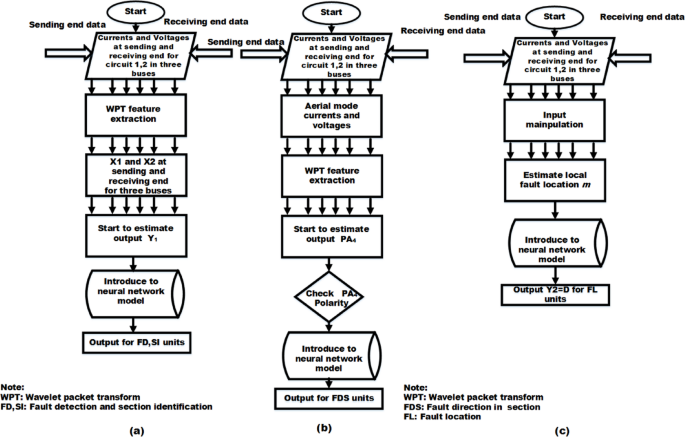
Flowchart of the suggested fault diagnosis method: (a) FD, fault section identification; (b) Fault direction in section; (C) Fault location.