Rapidly developing satellite remote sensing observations offer opportunities to develop data-driven large-scale spatiotemporal Chl_a prediction method. However, three major challenges must first be solved. First, temporal variations induced by complex physical and biogeochemical stressors are difficult to capture. Second, spatial heterogeneity and relationships are difficult to represent. Third, the high rates of missing satellite observations compromise the completeness of spatiotemporal variations of Chl_a, rendering these observations inadequate to use for accurate prediction.
STIMP is an AI-powered unified framework composed of two steps: 1) spatiotemporal satellite Chl_a data imputation pθ and 2) Chl_a prediction pΦ. By doing so, STIMP effectively reconstructs the complete spatiotemporal variations of Chl_a, X, from partial observations, Xob, subsequently providing accurate large-scale spatiotemporal predictions of Chl_a \(\tilde{{{{\bf{Y}}}}}\) across coastal oceans, such that:
$$p(\tilde{{{{\bf{Y}}}}}| {{{{\bf{X}}}}}^{ob})=\int_{{{{\bf{X}}}}}{p}_{{{\Phi }}}(\tilde{{{{\bf{Y}}}}}| {{{\bf{X}}}}){p}_{\theta }({{{\bf{X}}}}| {{{{\bf{X}}}}}^{ob})d{{{\bf{X}}}},$$
(3)
where \({{{{\bf{X}}}}}^{ob}\in {{\mathbb{R}}}^{T\times N}\), N denotes the number of positions and T denotes the length of time series; \(\tilde{{{{\bf{Y}}}}}\in {{\mathbb{R}}}^{{T}^{{\prime} }\times N}\), \({T}^{{\prime} }\) denotes the predicted length.
We approximate Equation (3) by sampling a finite number of samples and using a summation form, which is formulated as:
$$p(\tilde{{{{\bf{Y}}}}}| {{{{\bf{X}}}}}^{ob})={\sum}_{{{{\bf{X}}}}}{p}_{{{\Phi }}}(\tilde{{{{\bf{Y}}}}}| {{{\bf{X}}}}){p}_{\theta }({{{\bf{X}}}}| {{{{\bf{X}}}}}^{ob}).$$
(4)
Here, several datasets X are generated by well-trained pθ(X∣Xob). Based on each dataset, we trained specific \({p}_{{{\Phi }}}(\tilde{{{{\bf{Y}}}}}| {{{\bf{X}}}})\). Using Rubin’s rules32, the final Chl_a prediction is obtained by averaging the prediction of specific \({p}_{{{\Phi }}}(\tilde{{{{\bf{Y}}}}}| {{{\bf{X}}}})\) based on different X. In this way, our STIMP method not only improves the overall predictive performance through accurate imputation of missing data but also provides confidence intervals to quantify the prediction uncertainties. More details of training \({p}_{{{\Phi }}}(\tilde{{{{\bf{Y}}}}}| {{{\bf{X}}}})\) and pθ(X∣Xob) can be found in the following two subsections.
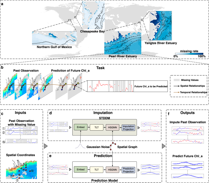
Spatiotemporal satellite Chl_a data imputation
We contrived a spatiotemporal denoising diffusion model (STDDM) that we applied to the imputation function, pθ(X∣Xob). STDDM is fundamentally a Denoising Diffusion Probabilistic Model (DDPM) specifically designed to approximate the spatiotemporal distribution of Chl_a conditioned on partial observations.
The imputation function conditioned on partial observation. Imputation function intends to leverage deep generative learning to approximate spatiotemporal distribution of Chl_a. The primary challenge in learning the imputation function lies in the complex spatiotemporal distribution of Chl_a, which is challenging to transform from easy-to-sample distribution using neural networks. Inspired by DDPM, we decompose the complex task into L simple tasks. We can manually set a sequence of data distributions perturbed by L levels of signal-to-noise ratio. The objective of each task is to improve the signal-to-noise ratio of the perturbed data distribution from \({\sigma }_{l}^{2}\) to \({\sigma }_{l-1}^{2}\), where 0 ≈ σL σL−1 σ0. The final complex spatiotemporal distribution of Chl_a is obtained by the joint distribution p(X, X1:L∣Xob) defined as a Markov chain with learned Gaussian transitions starting at an easy-to-sample distribution \(p({{{{\bf{X}}}}}_{L})={{{\mathcal{N}}}}({{{{\bf{X}}}}}_{L};{{{\bf{0}}}},{{{\bf{I}}}})\):
$${p}_{\theta }({{{\bf{X}}}}| {{{{\bf{X}}}}}^{ob})= \int\,p({{{\bf{X}}}},{{{{\bf{X}}}}}_{1:L}| {{{{\bf{X}}}}}^{ob})d{{{{\bf{X}}}}}_{1:L}= \int\,{p}_{\theta }({{{\bf{X}}}}| {{{{\bf{X}}}}}_{1:L},{{{{\bf{X}}}}}^{ob}){p}_{\theta }({{{{\bf{X}}}}}_{1:L}| {{{{\bf{X}}}}}^{ob})d{{{{\bf{X}}}}}_{1:L}\\ = \int\,p({{{{\bf{X}}}}}_{L}){p}_{\theta }({{{\bf{X}}}}| {{{{\bf{X}}}}}_{1},{{{{\bf{X}}}}}^{ob}){\prod}_{l=L}^{2}{p}_{\theta }({{{{\bf{X}}}}}_{l-1}| {{{{\bf{X}}}}}_{l},{{{{\bf{X}}}}}^{ob})d{{{{\bf{X}}}}}_{1:L}.$$
(5)
In contrast to the noise predictor in DDPM, STDDM is an original data predictor which is utilized in the learned Gaussian transitions pθ(Xl−1∣Xl, Xob). Because a time series of Chl_a data usually contain irregular noisy components, estimating the noise is challenging. Note that we can incorporate pθ(X∣X1, Xob) into pθ(Xl−1∣Xl, Xob) and X can be regarded as clean samples with a signal-to-noise ratio σ0. Specifically, we define the signal-to-noise ratio \({\sigma }_{l}^{2}={\bar{\alpha }}_{l}/(1-{\bar{\alpha }}_{l})\), where \({\bar{\alpha }}_{l}={\prod }_{i=1}^{l}{\alpha }_{i}\) and [α0, ⋯ , αL] is a manually defined noise schedule in which each element regulates the levels of added Gaussian noise to Xl−1. Then, the objective of the learned Gaussian transition in the l-th task is formulated as:
$${p}_{\theta }({{{{\bf{X}}}}}_{l-1}| {{{{\bf{X}}}}}_{l},{{{{\bf{X}}}}}^{ob})={{{\mathcal{N}}}}({{{{\bf{X}}}}}_{l-1};\frac{(1-{\bar{\alpha }}_{l-1})\sqrt{{\alpha }_{l}}}{1-{\bar{\alpha }}_{l}}{{{{\bf{X}}}}}_{l}+\frac{(1-{\alpha }_{l})\sqrt{{\bar{\alpha }}_{l-1}}}{1-{\bar{\alpha }}_{l}}{{{\bf{X}}}},\frac{(1-{\alpha }_{l})\sqrt{{\bar{\alpha }}_{l-1}}}{1-{\bar{\alpha }}_{l}}{{{\bf{I}}}}).$$
(6)
Unfortunately, the original spatiotemporal distribution of Chl_a, X, is unknown for pθ(Xl−1∣Xl, Xob). Hence, we contrive STDDM, an original data predictor, to approximate X with partial observation Xob and a perturbed Chl_a distribution, Xl, that is, p(X∣Xl, Xob). STDMM is learned by the following objective function:
$${\min }_{\theta }{{\mathbb{E}}}_{{{{{\bf{X}}}}}_{0}}{{\mathbb{E}}}_{{{{\mathcal{N}}}}({{{{\bf{X}}}}}_{l};\sqrt{{\bar{\alpha }}_{l}}{{{{\bf{X}}}}}_{0},(1-{\bar{\alpha }}_{l}){{{\bf{I}}}})}(| | STDD{M}_{\theta }({{{{\bf{X}}}}}^{ob},{{{{\bf{X}}}}}_{l})-{{{\bf{X}}}}| {| }^{2}),$$
(7)
In practice, however, three challenges remain in learning the STDMM. First, STDMM cannot differentiate between different subtasks using only Xob and Xl as input, leading to difficulties in optimization. To address this issue, we incorporate the task number l as the input to the STDMM. Second, due to we select N locations belong to the ocean as the Xob, STDMM cannot obtain location information, resulting in an inability to obtain spatial heterogeneity and relationships. We construct the spatial graph \({{{\bf{G}}}}\in {{\mathbb{R}}}^{N\times N}\) to maintain spatial relationships of these locations. By default, if latitude and longitude difference between location i and j are both less than 0.05°, we set Gij = 1. By doing so, STIMP can extract information from adjacent locations during the information aggregation of Heterogeneous Spatial Graph Neural Network (HSGNN). Third, we cannot obtain the true values for unobserved Chl_a as a supervised learning signal. As a compromise, we treat the observed data as X, and further mask part of X with M to obtain partial observations Xob ← (1 − M) ⊙ X, where ⊙ denotes the element-wise product. Because we focus on the performance of reconstructing the unobserved value, the corresponding objective function is given by:
$${\min }_{\theta }{{\mathbb{E}}}_{{{{\bf{X}}}}}{{\mathbb{E}}}_{{{{\mathcal{N}}}}({{{{\bf{X}}}}}_{l};\sqrt{{\bar{\alpha }}_{l}}{{{\bf{X}}}},(1-{\bar{\alpha }}_{l}){{{\bf{I}}}})}(| | {{{\bf{M}}}}\odot (STDD{M}_{\theta }({{{{\bf{X}}}}}^{ob},{{{{\bf{X}}}}}_{l},l,{{{\bf{G}}}})-{{{\bf{X}}}})| {| }^{2}),$$
(8)
The training process of STDDM is summarized in Algorithm 1.
Algorithm 1
Training Process of STIMP for imputation.
Input : A sample of training data, \({{{\bf{X}}}}\in {{\mathbb{R}}}^{T\times N}\); Spatial Graph, \({{{\bf{G}}}}\in {{\mathbb{R}}}^{N\times N}\); the number of denoising steps, L; the number of training iteration, M.
Output : Optimized STDDM
1. for s = 1 to M do
2. Get random mask M
3. Xob ← (1 − M) ⊙ X
4. Sample \(l \sim Uniform(1,2,\cdots \,,L),\epsilon \sim {{{\mathcal{N}}}}({{{\bf{0}}}},{{{\bf{I}}}})\)
5. Get perturbed value \({{{{\bf{X}}}}}_{l}\leftarrow \sqrt{{\bar{\alpha }}_{l}}{{{{\bf{X}}}}}^{ob}+\sqrt{1-{\bar{\alpha }}_{l}}\epsilon .\)
6. Estimate missing value with STDDMθ(Xob, Xl, l, G)
7. Update the gradient by ∇ ∣∣M ⊙ (STDDMθ(Xob, Xl, l, G) − X0)∣∣2
8. end
Reconstructing the missing values with the imputation function
Now we show how we generate missing Chl_a by leveraging the learned imputation function. During imputation, we reconstruct the missing values of satellite Chl_a data using the partial observation. Assuming that the STDDM training was good enough to accurately simulate p(X∣Xl, Xob), the final complex spatiotemporal distribution of Chl_a is obtained by progressively reducing the signal-to-noise ratio. Starting at samples XL from the Gaussian distribution, the signal-to-noise ratio can be reduced by getting samples from the following learned Gaussian transition, replacing X with STDDM(Xob, Xl, l, G) in Eq. (6):
$${{{{\bf{X}}}}}_{l-1}\leftarrow \frac{(1-{\bar{\alpha }}_{l-1})\sqrt{{\alpha }_{l}}}{1-{\bar{\alpha }}_{l}}{{{{\bf{X}}}}}_{l}+\frac{(1-{\alpha }_{l})\sqrt{{\bar{\alpha }}_{l-1}}}{1-{\bar{\alpha }}_{l}}STDDM\\ ({{{{\bf{X}}}}}^{ob},{{{{\bf{X}}}}}_{l},l,{{{\bf{G}}}})+\frac{(1-{\alpha }_{l})\sqrt{{\bar{\alpha }}_{l-1}}}{1-{\bar{\alpha }}_{l}}\epsilon$$
(9)
where \(\epsilon \sim {{{\mathcal{N}}}}({{{\bf{0}}}},{{{\bf{I}}}})\). We summarized the imputation in Algorithm 2.
Spatiotemporal Chl_a prediction
We predict the most probable length-\({T}^{{\prime} }\) sequence of Chl_a \(\tilde{{{{\bf{Y}}}}}\) with \({p}_{{{\Phi }}}(\tilde{{{{\bf{Y}}}}}| {{{\bf{X}}}})\). To achieve this goal, the data distributions in space and time are important and warrant careful consideration. Fortunately, we must obtain a complete spatiotemporal distribution of Chl_a X is obtained by imputing the Chl_a spatiotemporal satellite data, denoted by pθ(X∣Xob) in Eq. (3). We meticulously designed the network architecture to effectively capture spatial correlations and temporal dynamics.
First, we leverage a value embedding network with a 1 × 1 kernal convolutional layer to encode the information of historical observation of Chl_a, X:
$${{{\bf{H}}}}=Conv({{{\bf{X}}}}).$$
(10)
Then, STIMP separately captures the spatial and temporal relationship of the input H separately. First, the temporal features Htemp are learned by a temporal dependency learning module TLT:
$${{{{\bf{H}}}}}^{temp}=TLT({{{\bf{H}}}}),$$
(11)
Then, the spatial relationships and heterogeneity from the spatial graph, G, are further mined by HSGNN:
$${{{{\bf{H}}}}}^{spa}=HSGNN({{{{\bf{H}}}}}^{temp},{{{\bf{G}}}}).$$
(12)
Eventually, the predicted Chl_a is obtained using a two-layer fully connected neural network:
$$\tilde{{{{\bf{Y}}}}}={F}_{2}^{pre}(SiLU({F}_{1}^{pre}({{{{\bf{H}}}}}^{spa}))),$$
(13)
where SiLU is activation function.
The objective function of training \({p}_{{{\Phi }}}(\tilde{{{{\bf{Y}}}}}| {{{\bf{X}}}})\) is given by:
$${\min }_{{{\Phi }}}{{\mathbb{E}}}_{{{{\bf{X}}}},\tilde{{{{\bf{Y}}}}} \sim {p}_{{{\Phi }}}(\tilde{{{{\bf{Y}}}}}| {{{\bf{X}}}})}(| | {{{\bf{Y}}}}-\tilde{{{{\bf{Y}}}}}| {| }^{2}).$$
(14)
Algorithm 2
STIMP Imputation
Input : A sample of incomplete observed data, \({{{{\bf{X}}}}}^{ob}\in {{\mathbb{R}}}^{T\times N}\), with observation indicator, M; Spatial Graph, \({{{\bf{G}}}}\in {{\mathbb{R}}}^{N\times N}\); the number of diffusion steps, L; and the optimized STDDM.
Output : Imputed data X
1. Set \({{{{\bf{X}}}}}_{L} \sim {{{\mathcal{N}}}}(0,I)\)
2. For l = L to 1 do
3. \({{{{\bf{X}}}}}_{l-1}\leftarrow \frac{(1-{\bar{\alpha }}_{l-1})\sqrt{{\alpha }_{l}}}{1-{\bar{\alpha }}_{l}}{{{{\bf{X}}}}}_{l}+\frac{(1-{\alpha }_{l})\sqrt{{\bar{\alpha }}_{l-1}}}{1-{\bar{\alpha }}_{l}}STDDM({{{{\bf{X}}}}}^{ob},{{{{\bf{X}}}}}_{l},l,{{{\bf{G}}}})\)
4. \(\epsilon \sim {{{\mathcal{N}}}}(0,I)\)
5. \({{{{\bf{X}}}}}_{l-1}\leftarrow {{{{\bf{X}}}}}_{l-1}+\frac{(1-{\alpha }_{l})\sqrt{{\bar{\alpha }}_{l-1}}}{1-{\bar{\alpha }}_{l}}\epsilon\)
6. end
7. \({{{\bf{X}}}}\leftarrow \frac{(1-{\bar{\alpha }}_{0})\sqrt{{\alpha }_{1}}}{1-{\bar{\alpha }}_{1}}{{{{\bf{X}}}}}_{1}+\frac{(1-{\alpha }_{1})\sqrt{{\bar{\alpha }}_{0}}}{1-{\bar{\alpha }}_{1}}STDDM({{{{\bf{X}}}}}^{ob},{{{{\bf{X}}}}}_{1},1,{{{\bf{G}}}})\)
8.X ← M ⊙ Xob + (1 − M) ⊙ X
Network structures of STDDM
STDDM does not limit the network architecture. To make the model for suitable for spatiotemporal imputation, as shown in Supplementary Fig. S16c, we leveraged TLT and HSGNN to handle temporal and spatial relationships, respectively. Specifically, STDDM concatenates the time series of partial observation, Xob; perturbed values, Xl; diffusion step, l; and spatial graph, G as the input. STDDM utilizes a value embedding network with a 1 × 1 kernel convolutional layer to encode the information and outputs a d-dimensional latent representations:
$${{{\bf{H}}}}=Conv({{{{\bf{X}}}}}_{l}| | {{{{\bf{X}}}}}^{ob}),$$
(15)
where \({{{\bf{H}}}}\in {{\mathbb{R}}}^{L\times N\times d}\). The diffusion step, l, is specified by adding the Transformer sinusoidal position embedding (PE)55 to H:
$${{{{\bf{H}}}}}^{in}={{{\bf{H}}}}+DE(PE(l)),$$
(16)
where DE project consists of two fully connected layers and a Sigmoid Linear Unit (SiLU) function as the activation layer, and we broadcast this embedding vector over timesteps and positions L × N.
To comprehensively capture the global spatiotemporal and geographic relationship of input Hin, the temporal features, Htemp, is learned using the temporal dependency learning module TLT, and then the temporal features are aggregated through a spatial dependency learning module HSGNN:
$$\begin{array}{c}{{{{\bf{H}}}}}^{temp}=TLT({{{{\bf{H}}}}}^{in})\\ {{{{\bf{H}}}}}^{spa}=GN({{{{\bf{H}}}}}^{temp}+HSGNN({{{{\bf{H}}}}}^{temp},{{{\bf{G}}}})),\end{array}$$
(17)
where GN means Group Normalization56 to stabilize the training. More of the original information Htemp is preserved for Hspa.
Hout is obtained by leveraging the gated activation unit in CSDI37, which is formalized as:
$${{{{\bf{H}}}}}^{out}=sigmoid(Conv({{{{\bf{H}}}}}^{spa}))*tanh(Conv({{{{\bf{H}}}}}^{spa})),$$
(18)
where Conv is a convolutional layer with a 1 × 1 kernel. Finally, the predicted imputation target is obtained with
$${{{\bf{X}}}}={{{{\bf{F}}}}}^{imp}({{{{\bf{H}}}}}^{out}),$$
(19)
where Fimp is a fully connected layer.
Network structures of TLT
TLT is dedicated to effectively capturing the temporal relationships of Chl_a. In TLT, each element in the time series will compute attention with all other elements, thereby preserving and propagating essential information throughout the extended sequence55. The long- and short-term temporal dependencies captured by TLT significantly enhance the accuracy of large-scale spatiotemporal Chl_a imputations and predictions.
Specifically, TLT takes the representations of Chl_a from a time series \({{{{\bf{H}}}}}^{in}\in {{\mathbb{R}}}^{L\times N\times d}\) as input, yielding the enriched temporal representation \({{{{\bf{H}}}}}^{temp}\in {{\mathbb{R}}}^{L\times N\times d}\) by encoding the time dependency in Hin. Two key modules in TLT are the Multi-head Self-Attention (MSA) and Position-wise Feed-Forward (PFF). MSA is mainly in charge of capturing temporal relationships and PFF endows the model with nonlinearity. We mathematically represent the overall procedure of TLT as a function as follows:
$${{{{\bf{H}}}}}^{temp}=LN(PFF(LN(MSA({{{{\bf{H}}}}}^{in})))),$$
(20)
where LN is the standard normalization layer. The key component in MSA is self-attention (SA) along the temporal dimension L, which is defined as follows,
$$SA(Q,K,V)=softmax(\frac{Q{K}^{T}}{\sqrt{d}})V,$$
(21)
where Q = HinW Q; K = HinW K; V = HinW V represent the queries, the keys, and the values, respectively, which are converted from Hin, WQ, WK, and \({W}^{V}\in {{\mathbb{R}}}^{d\times d}\) are learnable projection parameters. Essentially, MSA computes the dot product of Qi and Kj to generate a weight that measures the relevance between Chl_a at times i and j.
MSA utilizes several SA layers: MSA(Hin) = Concat(h1, h2, ⋯ , hn)WO + Hin where hi = SA(Q, K, V). The residual is introduced to preserve more original Chl_a information. The added PFF networks consist of a fully connected layer and a Rectified Linear Unit(ReLU) function as and activation layer.
Network structures of HSGNN
To leverage the spatial dependency of Chl_a, we contrived HSGNN to obtain the enriched spatiotemporal representation, \({{{{\bf{H}}}}}^{spa}\in {{\mathbb{R}}}^{L\times N\times d}\) by encoding the spatial dependency in Htemp with the assistance of G:
$${{{{\bf{H}}}}}^{spa}={{{{\bf{F}}}}}^{spa}({{{\bf{W}}}}\cdot {{{{\bf{H}}}}}^{temp}\cdot {{{\bf{G}}}}).$$
(22)
As shown in Supplementary Fig. S16d (a), the time series exhibits spatial heterogeneity, with significantly different means and variances of Chl_a at different locations. Hence, the same parameter W for different locations does not meet the requirements.
However, it is impractical to design a separate set of parameters for each different position. For the spatial parameter space, \({\theta }^{spa}\in {{\mathbb{R}}}^{N\times d\times d}\), directly optimizing this parameter spaces brings huge computational burden and data demand, especially when N is large. Instead, we provide a simple yet effective way to maintain a small parameters pool, \({{{\bf{P}}}}\in {{\mathbb{R}}}^{k\times d\times d}\), which contains k parameter prototypes. k is defined to be much smaller than N. We can generate a spatial embedding \({{{\bf{Q}}}}\in {{\mathbb{R}}}^{k\times N}\) as a query for all positions, and we can obtain a location-specific parameter using a weighted combination of the parameter prototypes:
$${{{{\bf{W}}}}}^{spa}={{{{\bf{Q}}}}}^{T}\cdot {{{\bf{P}}}}.$$
(23)
Because spatial heterogeneity is mainly reflected in the mean and variance of the Chl_a time series across different positions, we generate a query, Q, for all positions according to each location, \(L\in {{\mathbb{R}}}^{1\times N}\), mean, \(\mu \in {{\mathbb{R}}}^{1\times N}\), and variance, \(\varsigma \in {{\mathbb{R}}}^{1\times N}\):
$${{{\bf{Q}}}}={{{{\bf{H}}}}}^{T}\left[\begin{array}{c}L\\ \mu \\ \varsigma \\ \end{array}\right],$$
(24)
where \({{{\bf{H}}}}\in {{\mathbb{R}}}^{3\times k}\). In doing so, the learned parameter reduces from \({\theta }^{spa}\in {{\mathbb{R}}}^{N\times d\times d}\) to \({{{\bf{H}}}}\in {{\mathbb{R}}}^{3\times k}\) and \({{{\bf{P}}}}\in {{\mathbb{R}}}^{k\times d\times d}\).
Then, we leverage \({{{{\bf{W}}}}}^{spa}\in {{\mathbb{R}}}^{N\times d\times d}\) to replace the original parameters \({{{\bf{W}}}}\in {{\mathbb{R}}}^{d\times d}\) in Equation (22), introducing the spatial heterogeneity using location specific parameters:
$${{{{\bf{H}}}}}^{spa}={{{{\bf{F}}}}}^{spa}({{{{\bf{W}}}}}^{spa}\cdot {{{{\bf{H}}}}}^{temp}\cdot {{{\bf{G}}}}),$$
(25)
where Fspa is a fully connected network. Now, each position obtains information from an adjacent position through Htemp ⋅ G. Meanwhile, location-specific parameters, Wspa, are utilized to embed the spatial heterogeneity into Hspa. As shown in Supplementary Fig. S16d, we leveraged the learned spatial heterogeneous embedding Q to partition the Pearl River Estuary. The results of the partition were generally consistent with the the isobaths at 30 m and 50 m below sea level, showing that STIMP indeed captured the spatial heterogeneity of different locations in the Pearl River Estuary.
More training details
STIMP employs Adam for stochastic optimization during model training. By default, the number of training epochs in STIMP is 500 and 200 for imputation and prediction respectively, with learning rate lr = 0.0001 and a weight decay parameter λ = 0.00001.
Computational demands
We computed the computational demands of STIMP, including FLOPs (floating-point operations), MACs (multiply-add operations) and Parameters, with Calflops (https://github.com/MrYxJ/calculate-flops.pytorch.git) on Pearl River Estuary. Moreover, we recorded the GPU memory usage of STIMP. Note that we set the batch size of training data is equal to 1 when calculating FLOPs, MACs and GPU memory, which means the minimum computational requirements for running STIMP. The hardware requirements analysis in Table 1 reveals that STIMP maintains low GPU memory demands (≥1.5 GB), compatible with obsolete consumer hardware, including NVIDIA’s GTX 1050 (2016 release). This highlights the framework’s practical deployability even with limited computational resources.
Table 1 Computational demands of STIMP