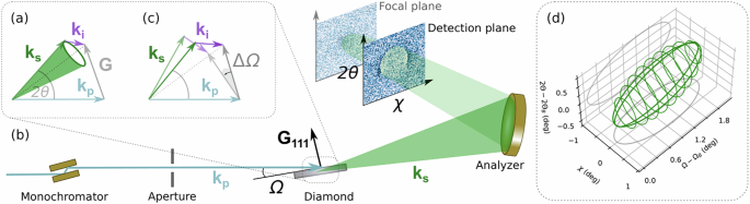
Experimental setup
We performed the experiment at the large solid-angle spectrometer of beamline ID20 at ESRF26. The setup’s geometry follows Fig. 1c. The incident beam passes through a Si(111)-double-crystal monochromator, limiting its spectral bandwidth to ~1 eV (FWHM) around the pump photon energy of ℏωp = 9.79 keV at a fluence of ~1013 ph/s. As our sample, we use a diamond single-crystal of 1 mm thickness and (111) surface-cut. This is initially positioned for its symmetric (111) Bragg-reflection at Ω= θB = 17.91° (nominal calibration) and subsequently aligned to fulfill phase-matching conditions at Ω= θB + ∆Ω (measurements for ∆Ω = [0.27,…, 1.87°], see Fig. 5 below). We filter for the XPDC signal using a Si(660) crystal analyzer, which is spherically bent with a 1 m curvature radius. It is positioned at a (vertical) scattering angle of 2θB in ~ 1 m distance downstream of the sample (viz., the so-called Rowland geometry). The analyzer is aligned close to back-reflection (θanalyzer).
Fig. 5: Measurements of the XPDC cone extended.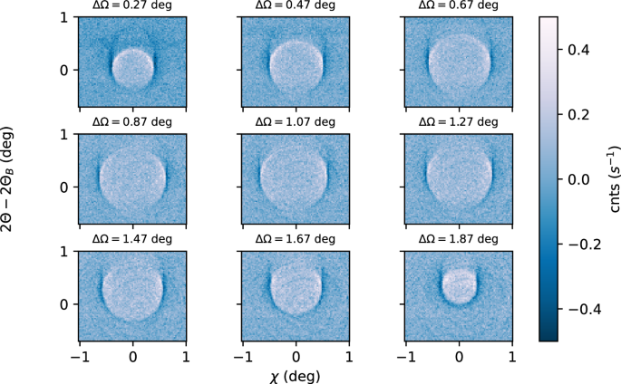
All scattering images from Fig. 2d [main text] arranged in 2D51. Scattering angles (2θ, χ) are fixed to the same range for all frames; individual sample angle ∆Ω is indicated above each plot.
Angle calibration
We calibrate the 2-dimensional detector images from pixels to scattering angles [deg] by means of the sample’s (111) Bragg-reflection. This locates the (nominal) scattering angle 2θ = 2θB, corresponding to pixel 117 vertically, and also defines the scattering plane around χ = 0, corresponding to pixel 79 horizontally. The scale relative to this reference is obtained by moving the detection-arm (i.e., the assembly including analyzer and detector) along 2θ by ±2°. We convert the pixel positions that the Bragg reflex traverses on the detector during this movement into the calibration: 1 pixel ≜ 0.0205°.
This holds for both the χ – and the 2θ-axes, as the pixels are quadratic.
$$2\theta \left[{{{\rm{deg}}}} \right]=\left(2\theta \left[{{{\rm{pixel}}}}\right]-117\, {{{\rm{pixel}}}}\right)\times 0.0205\, {{{\rm{deg}}}} /{{{\rm{pixel}}}}$$
(4)
$$\chi \left[{{{\rm{deg}}}} \right]=\left(\chi \left[{{{\rm{pixel}}}}\right]-79\,{{{\rm{pixel}}}}\right)\times 0.0205\,{{{\rm{deg}}}} /{{{\rm{pixel}}}}.$$
(5)
Mapping to momentum transfer
Mapping from scattering angles (2θ, χ) to momentum transfer ℏq = ℏ(kp–ks) proceeds in a system of spherical coordinates. The pump beam defines the polar axis along kp = ωp/cez, where c is the speed of light in vacuo and ez the unit vector along z. The signal photon’s ks is fully determined by its magnitude |ks | = ωs/c as well as the scattering angles 2θ = θs for its azimuth and
$$\chi \to \phi s=\left(\chi -{{{\pi }}}/2\right)\left(\sin 2\theta \right)-1+{{{\pi }}}/2$$
(6)
for its polar angle. Following Eq. (3) [main text], q relates to the photonic level of the TLS via
$${{{{{\bf{k}}}}}^{{{{\rm{eff}}}}}}_{{{{\gamma }}}}={{{\bf{q}}}}+{{{\bf{G}}}}={{{{\bf{k}}}}}_{{{{\bf{p}}}}}-{{{{\bf{k}}}}}_{{{{\bf{s}}}}}+{{{\bf{G}}}}$$
(7)
analogous to the phase-matching condition. Writing the reciprocal lattice vector in the same coordinate system
$${{{\bf{G}}}}={\omega }_{p}{c}^{-1}\sin {\theta }_{B}\left(\begin{array}{c}0\\ \cos \theta B+\Delta \Omega \\ \sin \theta B+\Delta \Omega \end{array}\right),$$
(8)
we can compute \({{{{\bf{k}}}}}_{{{\gamma }}}^{{{{\rm{eff}}}}}\) for all scattering angles and evaluate the pertaining dispersion relations ωγ(q) or E±(ωγ) numerically. The prefactor in Eq. (8) reflects Bragg’s law.
Background subtraction
The nonlinear conversion signal is imprinted on top of a stronger background, approximately within a ratio of 1/10. This background consists predominantly of (diffuse) Compton-scattering, which is further modulated by aberrations due to the crystal optics. To expose the XPDC signal, we subtract a scaled back-ground image from each recorded frame individually:
$${{{Frame}}_{{corrected}}}^{\left(i\right)}{={Frame}}^{\left(i\right)}-\left({{Frame}}^{\left({offPM}\right)} * \frac{\sum {{Frame}}^{\left(i\right)}}{\sum {{Frame}}^{\left({offPM}\right)}}\right)$$
(9)
For that purpose we acquire a scattering image off the phase-matching condition, viz., Frame(off PM), that contains no XPDC, but still features the background with imprints of the analyzer. Scaling is based on the total (background) counts per frame, i.e., Frame(i), and varies slowly across the phase-matching range.
Polarization-imprint on coupling V
We have postulated previously that parametric conversion from X-ray to optical photons will exhibit circumferential modulations of its scattering cones that relate to the polarization of the idler photons24. Confirming the same pattern experimentally in the EUV-case, we seek to incorporate this characteristic into our TLS-model as well. The transversality constraint from ref. 23 translates into our simplified coupling scheme as:
$$V\to V\times \left(1-{\left|{\hat{{{{\bf{k}}}}}}_{{{{\rm{\gamma }}}}}^{{{{\rm{eff}}}}}\cdot \hat{{{{\bf{G}}}}}\right|}^{2}\right).$$
(10)
Angular variations derive from the orientation of the idler photon’s wavevector \({{{{\bf{k}}}}}_{{{\gamma }}}^{{{{\rm{eff}}}}}\) relative to the reciprocal lattice vector G, represented through their respective unit vectors.
Using the modulation (10) in our simulations, we find excellent agreement with measured data in Fig. 4 [main text] (cf. minima around χ = 0), thus establishing first evidence for a non-trivial polarization dependence also in the case of polaritonic XPDC. In the extended data below (Fig. 6), we illustrate how the polarization imprint can also be simulated for the other cases of Fig. 2a–c [main text]. While the first column reproduces the earlier experimental images (for sample detunings of ∆Ωa = 0.47°, ∆Ωb = 1.07° and ∆Ωc = 1.87°, respectively), the second column juxtaposes the TLS simulations with coupling according to Eq. (10). For comparison, we also include a simplified version of constant, isotropic coupling in the third column of extended data Fig. 6. Finally, its fourth column visualizes the phase-matching condition for each case. This influences the signal via Eq. (10), rendering it predominantly sensitive to EUV-quanta that are polarized in the same direction as the reciprocal lattice vector G. As such, all side-lobes of the XPDC cones (i.e., for phasematching \({{{{\bf{k}}}}}_{{{\gamma }}}^{{{{\rm{eff}}}}}\) out of plane) show pronounced signal strength, because there is a component of its polarization along G to be imaged. In contrast, the polariton’s propagation direction (\({{{{\bf{k}}}}}_{{{{\boldsymbol{\gamma }}}}}^{{{{\bf{eff}}}}}\)) at the upper or lower point of the cone may align with G, rendering its polarization largely orthogonal. This results in signal suppression, which is most visible in Fig. 2b around χ = 0. Similarly, for the conditions shown in Fig. 2a or c, \({{{{\bf{k}}}}}_{{{{\boldsymbol{\gamma }}}}}^{{{{\bf{eff}}}}}\) aligns with G at the lower- or uppermost phase-matching point, respectively. Again, this leads to signal suppression – while on each opposite side of the cone, the EUV-idler’s polarization is allowed to be parallel to G, giving rise to strong signal and an overall horseshoe-shape.
Fig. 6: Polarization imprint on the XPDC cone.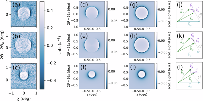
Juxtaposition of measured XPDC signal cones at different rocking angles (left column; a–c) with respective simulations that include (center-left; d–f) or disregard (center-right; g–i) polarization effects of the EUV-idler. The associated phase-matching conditions are sketched in the right-most column (j–l).
The effect merits future investigation, concerning its interplay with more complex dielectric structures.
Theoretical motivation of the TLS-model
To trace the imprint of polaritonic effects on XPDC, we base our description on the dynamic structure factor for inelastic X-ray scattering (IXS)37, which we express in atomic units below:
$$S({{{\bf{q}}}},\omega )=\frac{1}{2\pi }{\int }_{-\infty }^{\infty }{dt}{e}^{{{{\rm{i}}}}\omega t}\int {d}^{3}x\int {d}^{3}{x}^{{\prime} }{e}^{-{{{\rm{i}}}}{{{\bf{q}}}}\cdot ({{{\bf{x}}}}-{{{{\bf{x}}}}}^{{\prime} })}\left\langle \hat{n}({{{\bf{x}}}},t)\, \hat{n}({{{{\bf{x}}}}}^{{\prime} },0)\right\rangle .$$
(11)
Focusing on the density-density correlator and expanding its intermediate states, we write
$$\left\langle \hat{n}({{{\bf{x}}}},t)\, \hat{n}({{{{\bf{x}}}}}^{{\prime} },0)\right\rangle \approx {\sum }_{{n}_{i}}^{{{{\rm{VB}}}}}{\sum }_{{{{{\bf{k}}}}}_{i}}^{1.{{{\rm{BZ}}}}} |0 > ,$$
(12)
where we have expressed electronic states as Bloch-waves and—unconventionally for S(q,ω)—included additional photonic degrees of freedom in terms of initially unoccupied Fock states |0>. Assuming phase-matching conditions and the dipole-approximation for the EUV-light-matter interaction48 all terms remain approximately diagonal in their respective k-space coordinates, which is reflected in the single summation over ki. The central matrix element \( {|}0 > \) consists of highly excited electronic states, which would conventionally be considered only for their role as Compton-electrons—evolving quasi-free at ~100 eV. Within the band structure, however, such an electron also has a finite chance of returning to its initial valence-band state (now a hole at \({\varphi }_{{n}_{i},{{{{\bf{k}}}}}_{i}}\)) by emission of a 100 eV photon. This photonic coupling of states gives rise to the EUV-polariton. Notwithstanding the large number of overall bands nm, there will typically be only very few (if any) states that match the photonic resonance at \(100\,{{{\rm{eV}}}}={\epsilon }_{{n}_{m},{{{{\bf{k}}}}}_{i}}-{\epsilon }_{{n}_{i},{{{{\bf{k}}}}}_{i}}\). For our modeling, we will focus on those pairs of states \({\varphi }_{{n}_{m},{{{{\bf{k}}}}}_{i}}\); \({\varphi }_{{n}_{i},{{{{\bf{k}}}}}_{i}}\), that are closest to the transition at each k-point. This effectively establishes a set of near-resonant two-level systems (TLS) with Hamiltonians deriving from
$$\hat{H}={\hat{H}}_{{{{\rm{Bloch}}}}}+{\hat{H}}_{{{{\rm{phot}}}}}+{\hat{H}}_{{{{\rm{interaction}}}}}$$
(13)
$$\Rightarrow \left(\begin{array}{cc}{\epsilon }_{{n}_{i},{{{{\bf{k}}}}}_{i}} & 0\\ 0 & {\epsilon }_{{n}_{m},{{{{\bf{k}}}}}_{i}}\end{array}\right)+\left(\begin{array}{cc}{\omega }_{{{{{\bf{k}}}}}_{\gamma }} & 0\\ 0 & 0\end{array}\right)+\left(\begin{array}{cc}0 & V({n}_{i},{{{{\bf{k}}}}}_{i})\\ {V}^{{{\dagger}} }({n}_{i},{{{{\bf{k}}}}}_{i}) & 0\end{array}\right),$$
(14)
including coupling elements \(V({n}_{i},{{{{\bf{k}}}}}_{i})={\sum}_{{{{{\bf{k}}}}}_{\gamma }}^{{PM}}{\sum }_{\lambda }\sqrt{\frac{2\pi }{V{\omega }_{{{{{\bf{k}}}}}_{\gamma }}}} \) based on the interaction terms of ref. 48, with the range of photon momenta being constraint by phase-matching (PM). Equivalent reductions to resonant few-level emitters are at the core of many polaritonic descriptions—typically leading to Tavis-Cummings or Dicke-type models (see, e.g., ref. 14). We choose to diagonalize each k-point and frequency individually, leading to the well-known eigenenergies
$${E}_{\pm }({n}_{i},{{{{\bf{k}}}}}_{i})= \frac{({\epsilon }_{{n}_{m},{{{{\bf{k}}}}}_{i}}-{\epsilon }_{{n}_{i},{{{{\bf{k}}}}}_{i}})+{\omega }_{{{{{\bf{k}}}}}_{\gamma }}}{2} \\ \pm \sqrt{\frac{1}{4}({({\epsilon }_{{n}_{m},{{{{\bf{k}}}}}_{i}}-{\epsilon }_{{n}_{i},{{{{\bf{k}}}}}_{i}})-{\omega }_{{{{{\bf{k}}}}}_{\gamma }}})^{2}+{\left|V({n}_{i},{{{{\bf{k}}}}}_{i})\right|}^{2}}.$$
(15)
The corresponding eigenstates are obtained by the transformation
$$\begin{array}{c}\hat{T}\left({n}_{i},{{{{\bf{k}}}}}_{i}\right)\left|{\varphi }_{{n}_{m},{{{{\bf{k}}}}}_{i}}\right. > \left|0\right. > ={\sum }_{\pm }{c}_{e\pm }({n}_{i},{{{{\bf{k}}}}}_{i})\left|{\phi }_{\pm }^{{{{\rm{pol}}}}}({n}_{i},{{{{\bf{k}}}}}_{i}) > \right.\\ {{{\rm{with}}}}\,{c}_{e\pm }\left({n}_{i},{{{{\bf{k}}}}}_{i}\right)={\left(1+\frac{{\left|V\left({n}_{i},{{{{\bf{k}}}}}_{i}\right)\right|}^{2}}{({E}_{\pm }{({n}_{i},{{{{\bf{k}}}}}_{i})-{\omega }_{{{{{\bf{k}}}}}_{\gamma }}})^{2}}\right)}^{-\frac{1}{2}},\end{array}$$
(16)
which also transforms the original matrix element into
$$ \, |0 \, > ={\sum}_{\pm }{\left|{c}_{e\pm }\left({n}_{i},{{{{\bf{k}}}}}_{i}\right)\right|}^{2}{e}^{-i{E}_{\pm }\left({n}_{i},{{{{\bf{k}}}}}_{i}\right)t}$$
(17)
Combining Eqs. (1), (2) and (7), the dynamic structure factor near phase-matching (PM) becomes
$${S}^{{{{\rm{pol}}}}}({{{\bf{q}}}},\omega )= \frac{1}{{V}_{\diamond }}{\sum}_{{n}_{i}}^{{{{\rm{VB}}}}}{\sum}_{{{{{\bf{k}}}}}_{i}}^{1.{{{\rm{BZ}}}}}\left({\left|\int {d}^{3}x{e}^{-{{{\rm{i}}}}{{{\bf{qx}}}}} \right|}^{2}\right. \\ \left.{\sum}_{{{{{\bf{k}}}}}_{\gamma }}{\sum}_{\pm }{\left|{c}_{e\pm }\left({n}_{i},{{{{\bf{k}}}}}_{i}\right)\right|}^{2}\delta \left({E}_{\pm }\left({n}_{i},{{{{\bf{k}}}}}_{i}\right)-\omega \right)\right)$$
(18)
This represents the sum of partial scattering factors from all initial electronic states \({\varphi }_{{n}_{i},{{{{\bf{k}}}}}_{i}}\) – each dressed by a TLS, subject to energy conservation. Interpreting the summation as an average, we approximate the result as a single, effective TLS that dresses the overall dynamic structure factor with its Hopfield coefficients \({c}_{e\pm }\):
$${S}^{{{{\rm{pol}}}}}({{{\bf{q}}}},\omega )\approx {S}^{{{{\rm{IXS}}}}}({{{\bf{q}}}},\omega )\cdot {\sum}_{\pm }{\left|{c}_{e\pm }\right|}^{2}{e}^{-{({E}_{\pm }-\omega )}^{2}/{2\Gamma }_{{{{\rm{in}}}}}^{2}}$$
(19)
The single, effective two-level system marks the starting point for our main discussion. It is governed by the Hamiltonian of Eq. (M8), where ωe is the average transition energy and ωγ the average frequency of coupled photonic modes. Any relative variation within a sector is taken to be small and accounted for by an intrinsic broadening factor Γin, while the overall coupling of electronic and photonic sectors is now mediated by the collective coupling strength V.
Scattering yield from TLS-model
In order to connect our effective model to the observable scattering yield, we first relate \({S}^{{{{\rm{pol}}}}}({{{\bf{q}}}},\omega )\) to the double-differential scattering cross section of regular inelastic X-ray scattering (IXS)40 as follows
$$\frac{d{\sigma }^{{{{\rm{pol}}}}}}{d{\Omega }_{s}d{\omega }_{s}}={\left(\frac{d\sigma }{d{\Omega }_{s}}\right)}_{{Th}}\frac{{\omega }_{s}}{{\omega }_{p}}{S}^{{{{\rm{pol}}}}}\left({{{\bf{q}}}},{\omega }_{p}-{\omega }_{s}\right),$$
(20)
with the Thomson cross section (…)Th governing the proportionality40. After convoluting Eq. (20) with the incident fluence as well as the (Gaussian-modeled) transmission function of the analyzer-setup, we integrate for the scattering yield per pixel (i.e., covering (20.5 mdeg)2):
$${Y}_{{pix}}=p\cdot {\sum}_{\pm }{\left|{c}_{e \pm }\right|}^{2}{e}^{-{\left({{\hslash }}\Delta {\omega }_{{an}}-{E}_{\pm }\right)}^{2}/2({{\hslash }}{\Gamma })^{2}}.$$
(21)
Both E± and ce± are implicit functions of the scattering angles 2θ and χ at each point of evaluation. The overall bandwidth Γ as well as the energy-loss determined by the analyzer ∆ωan ~ ωγ are left as fitting parameters for simplicity, while the overall prefactor p is obtained from intrinsic background scattering (see below). Note that we have re-instated ℏ starting from Eq. (21).
Fitting procedure
We, consistently, resort to background-subtracted data for fitting, using Yfit=Ypix−Ybg. The pertinent background consists of inelastic (Compton) scattering and is captured by our Eq. (8) in the limit Spol(q, ω) →SIXS(q, ω). For regions of q-space away from polaritonic phase-matching. This translates onto Eq. (21) as
$${{{\mathrm{lim}}}}_{n\to \infty }{Y}_{{pix}}\left({{{{\rm{\omega }}}}}_{{{{\rm{\gamma }}}}}\right)={Y}_{{BG}}=p{e}^{-{\left(-\Delta {\omega }_{{an}}-{\omega }_{e}\right)}^{2}/2{\Gamma }^{2}}.$$
(22)
and automatically determines the prefactor p.
Binning the 2D data in a line-out along χ of width 7 pixel [see main text], we fit Yfit using the curve fit-routine from the freely-available python-package scipy.optimize. The result is shown in Fig. 4 [main text], with the underlying parameters determined to be: ℏωe = 98.36 ± 0.39 eV, V = 0.82 ± 0.08 eV, ℏΓ = 1.64 ± 0.22 eV and for the setup ℏΔωan = 99.90 ± 0.22 eV. The latter refines our knowledge of the difference ℏ(ωp − ωs) ≈ 100 eV. We assess the quality of the fitting by estimating the uncertainty by its reduced Χ2 ≈ 2.1, which is based on the counting error and indicates good agreement.
We note that the line shape could also be fitted by the Fano-formula49 on a phenomenological basis. This was done by Tamasaku et al. under similar conditions, suggesting an interference between Compton scattering and XPDC35. However, these processes should not interfere quantum mechanically (see also Tamasaku et al.50), which renders a Fano-model inapplicable. In contrast, our polaritonic interpretation reconciles both processes and yields Eq. (15) to describe the full, hybridized phenomenon.