Gradient indices from dielectric environment engineering
The propagation of polaritons is significantly influenced by the surrounding dielectric environment, particularly the dielectric permittivities of the substrate (εsub) and superstrate (εsup). We illustrate this by considering phonon polaritons (PhPs) in hexagonal boron nitride (hBN) and comparing two superstrates, air and PMMA. The dispersion relations for these systems are shown in Fig. 2a, derived from a waveguide-like eigenequation for a three-layer structure (see Supplementary Note 1 and Supplementary Fig. 1), with the hBN thickness (dhBN) fixed at 50 nm. Notably, the PMMA superstrate results in a higher in-plane momentum within the frequency range between the transverse optical (ωTO, 1340 cm−1) and longitudinal optical phonon frequencies (ωLO, 1630 cm−1) of hBN, corresponding to the type II Reststrahlen band. This effect arises from PMMA’s larger dielectric permittivity (εPMMA > εair) as depicted in Supplementary Fig. 2. Simulation results in the insets of Fig. 2a confirm that a PMMA superstrate enables a shorter polariton wavelength (λp) at a given frequency (ω = 1500 cm−1).
Fig. 2: Gradient effective refractive indices enabled by dielectric environment engineering.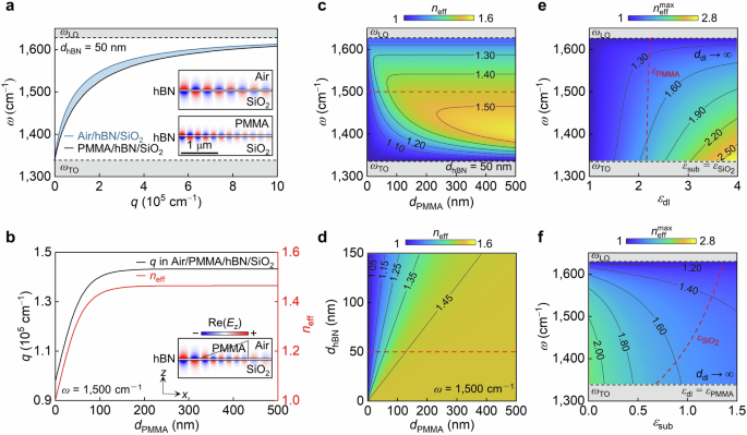
a Calculated dispersion relations of phonon polaritons in air/hBN/SiO2 and PMMA/hBN/SiO2 three-layer structures. Insets show simulated field distributions at the frequency (ω) of 1500 cm−1, with the hBN slab thickness (dhBN) set to 50 nm. b Polariton momentum (q) and effective refractive index (neff) as a function of PMMA thickness (dPMMA) in an air/PMMA/hBN/SiO2 four-layer structure. Inset shows the gradually decreasing polariton wavelengths across a PMMA taper. c Calculated neff as a function of dPMMA at different frequencies. d Tuning neff through adjustments in both dhBN and dPMMA. Dependence of the maximum refractive index (\({n}_{{{{\rm{eff}}}}}^{\max }\)) on the dielectric permittivities of the dielectric layer (εdl, e) and the substrate (εsub, f), under the approximation of the infinite dielectric layer thickness \(\left({d}_{{{{\rm{dl}}}}}\to {\infty }\right)\). Red curves respectively indicate the dielectric permittivities of PMMA (εPMMA) and SiO2 (\({\varepsilon }_{{{{\rm{Si}}}}{{{{\rm{O}}}}}_{2}}\)) employed in theoretical analysis.
When an hBN slab is overlaid with a PMMA layer of finite thickness (dPMMA), the polariton dispersion in this four-layer structure lies between those of the three-layer structures with either air or PMMA as the superstrate, as indicated by the blue region in Fig. 2a. The PMMA thickness thus serves as a key tuning parameter for continuously engineering polariton dispersions. As illustrated in Fig. 2b, when dPMMA = 0, the system resembles a three-layer structure with an air superstrate, while increasing dPMMA progressively elevates q, approaching the value associated with a PMMA superstrate. This trend is further supported by the simulation result in the inset of Fig. 2b, where λp gradually decreases along a PMMA taper.
The dPMMA-dependent dispersions of PhPs offer a promising strategy for designing refractive polaritonic lenses with gradient neff, as shown in Fig. 2c. A similar effect has also been observed in PMMA/gold and SiO2/graphene structures that rely on surface-confined plasmon polaritons32,34,35,37. By contrast, we employ PhPs supported by polar dielectrics, which exhibit lower losses in the mid-infrared range, facilitating more efficient visualisation of near-field distributions at room temperature (see below). Furthermore, unlike surface modes, PhPs in hBN are volume-confined modes, with their electromagnetic fields concentrated inside the thin slab. This property renders neff thickness dependence, with thinner hBN slabs leading to a more rapid increase in neff as dPMMA increases, as shown in Fig. 2d. However, the \({n}_{{{{\rm{eff}}}}}^{\max }\) is solely determined by the dielectric permittivities of the system, as given by:
$${n}_{{{{\rm{eff}}}}}^{\max }\approx \frac{{\varepsilon }_{{{{\rm{sub}}}}}+{\varepsilon }_{{{{\rm{PMMA}}}}}}{{\varepsilon }_{{{{\rm{sub}}}}}+{\varepsilon }_{\sup }}$$
(1)
at the frequency close to ωTO of hBN (Supplementary Note 1). Specifically, \({n}_{{{{\rm{eff}}}}}^{\max }\) can reach up to 1.69 for both the hBN slab (dhBN = 50 nm) and hBN monolayer supported by a SiO2 substrate (Supplementary Fig. 3). Even a higher neff could be achieved in polaritonic systems consisting of different materials, as demonstrated by the calculated neff as a function of the permittivities of the dielectric layer (εdl, Fig. 2e) and the substrate (Fig. 2f). These results outline a clear strategy for designing gradient polaritonic lenses through careful parameter selection.
Lithography-free approach for gradient polaritonic lenses
Previous methods for fabricating gradient polaritonic lenses primarily rely on grey-scale EBL, which involves patterning a spin-coated photoresist film to create spatially varying thicknesses after the lift-off process34. This approach requires precise control over the lithographic dose, particularly for nanoscale structures, which complicates the fabrication process. To address these challenges and enhance fabrication efficiency, we introduce a lithography-free method that utilises controlled melting of pre-prepared polymer microspheres. As illustrated schematically in Fig. 3a, a drop of PMMA microsphere suspension is deposited onto a SiO2/Si substrate supporting hBN slabs. After solvent evaporation, the microspheres adhere to the hBN surface. The sample is then heated to 250 °C and maintained for several hours, depending on the sizes of the hBN slabs and microspheres, allowing for the melting and controlled deformation of the PMMA microspheres. Upon cooling to room temperature, the melted PMMA solidifies into microstructures with gradient thicknesses, which can serve as gradient-index polaritonic lenses. See Methods for detailed fabrication procedures.
Fig. 3: Lithography-free approach to modelling PMMA caps.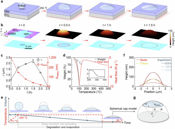
a Schematic illustration of the melting process of a PMMA sphere on the hBN surface. b Optical images of a PMMA sphere at each stage, with black circles marking the outlines of PMMA. The top panel displays corresponding atomic force microscopy images. c Measured radii (r) and heights (dPMMA) of the PMMA microstructure as a function of thermal treatment time (t). d Thermogravimetric analysis curve for the PMMA microsphere aqueous dispersion, with an inset zooming in on the evaporation of PMMA. The midpoint of the baseline step in heat flow determines the glass transition temperature (Tg). e Time-dependent temperature and volume diagram during thermal treatment. Top panel: schematic illustrations of representative morphologies at various stages, with grey dashed outlines indicating the previous stage for visual comparison. f Comparison of cross-sectional height profiles from experiments (blue), spherical cap models (red), and Luneburg lens theory (orange). g Sketch of a spherical cap within a hemisphere, with the radius of R. Because of the small aspect ratio of the PMMA microstructure (dPMMA/r « 1), its corresponding spherical cap is near the apex of the hemisphere with a small contact angle (θ).
The morphological evolution of a PMMA microsphere with an initial radius (r0) of 0.6 μm was investigated using optical microscopy and atomic force microscopy (AFM). Figure 3b displays optical microscopy images (bottom panel) alongside corresponding AFM profiles (top panel) of a PMMA microsphere on an hBN slab at various time intervals, revealing its deformation during thermal treatment. This behaviour is reminiscent of a water droplet spreading on a hot hydrophilic surface. Figure 3c quantifies the evolution, showing an initial increase in lateral radius followed by a subsequent reduction, accompanied by a monotonic decrease in height. These trends are further supported by volume (V) measurements shown in Supplementary Fig. 4. Additional experiments with finer temporal resolution on two other samples are provided in Supplementary Fig. 5. While the total evaporation time depends on microsphere size, all samples exhibit a consistent deformation pattern: an initial rapid lateral expansion within the first minute, followed by a slower increase, and a pronounced shrinkage around 2 h. This consistency underscores the reproducibility and robustness of our fabrication method.
Thermogravimetric analysis (TGA) of the PMMA microsphere suspension in air (Fig. 3d) reveals a glass transition temperature (Tg) of ~71 °C, notably lower than that of bulky PMMA (100–120 °C), due to the size-dependent Tg of PMMA38. Following an initial weight loss attributed to solvent evaporation, the sample mass remains stable up to 250 °C, indicating the onset of degradation and evaporation of PMMA. Combining the TGA data with the observed morphological evolution, we conclude that the final geometry of the PMMA microstructure is governed by the interplay between spreading and evaporation. Owing to the rapid heating rate, evaporation begins early in the process and proceeds concurrently with spreading. Therefore, the turning point in measured radius in Fig. 3c and Supplementary Fig. 5 does not correspond to the onset of evaporation, but rather the point at which volume loss due to evaporation begins to dominate over spreading-induced expansion. Conversely, the initial radius expansion reflects the dominance of spreading in the early stages. The competition between these two processes, compounded by the temperature-dependent viscosity of PMMA, renders quantitative modelling of this non-equilibrium transformation particularly challenging39. To provide qualitative insight, Fig. 3e schematically illustrates the morphological evolution of a PMMA microsphere during thermal treatment, alongside time-dependent profiles of temperature and volume.
Building on the observed morphological evolution of the PMMA microsphere, we develop a simple model to describe the geometry of PMMA microstructures during thermal treatment. The thicknesses of the PMMA microstructures, extracted from AFM profiles in Fig. 3b, are displayed in Fig. 3f (blue curves). Given the small aspect ratio of the obtained PMMA microstructures, where dPMMA/r « 1 with r being the lateral radius, we employ a spherical cap model to describe the geometry of PMMA microstructures as a function of the lateral radial distance (rd), defined by:
$${d}_{{{{\rm{PMMA}}}}}\left({r}_{{{{\rm{d}}}}}\right)=\sqrt{{R}^{2}-{{r}_{{{{\rm{d}}}}}}^{2}}-{d}_{{{{\rm{c}}}}}$$
(2)
where \(R=r/\sin (\theta )\) is the radius of the sphere, \({d}_{{{{\rm{c}}}}}=\sqrt{{R}^{2}-{r}^{2}}\) is the vertical distance between cap bottom and sphere centre, and θ represents the contact angle of the PMMA structure relative to the hBN surface, which is equal to half of the open angle of the spherical cap, as depicted in Fig. 3g. The calculated height profiles are represented by the red curves in Fig. 3f, which align well with experimental results. The fitting parameters are listed in Supplementary Table 1. This model offers a convenient means to predict and assess the evolution of PMMA microstructures during the controlled melting process.
Polaritonic lenses with gradient effective refractive indices
Our lithography-free and cost-effective method enables the in situ production of PMMA microstructures with variable height and controlled radius on the surfaces of polaritonic materials, facilitating the fabrication of polaritonic lenses with gradient neff. Taking the polaritonic Luneburg lens as an example, its refractive index distribution as a function of rd resembles that of an optical Luneburg lens, expressed as \({n}_{{{{\rm{eff}}}}}\left({r}_{{{{\rm{d}}}}}\right)=\sqrt{2-{\left({r}_{{{{\rm{d}}}}}/r\right)}^{2}}\) 31,32\(.\) Given its similar form to Eq. 2, such gradient indices are expected to be satisfied by the gradient height of our PMMA caps fabricated through our controllable melting method. Indeed, as shown in Fig. 3f, the as-prepared PMMA cap at t = 1.0 h closely matches the required geometry (orange curve) for a polaritonic Luneburg lens at ω = 1470 cm−1.
We use scattering-type scanning near-field optical microscopy (s-SNOM) to image polariton propagation in real space. This technique uses a sharp, apertureless metallic tip for the simultaneous excitation and detection of polaritons, along with topographic mapping. The real part of the second-harmonic near-field signal, Re(σ2), for a polaritonic lens is indicated by false colour in Fig. 4a, which is overlapped on the three-dimensional topography of the structure with dhBN = 89 nm. The cross-sectional height profile of the PMMA cap aligns well with the theoretical geometry for a polaritonic Luneburg lens at 1500 cm−1, resulting in concave interference patterns and a focal spot near the lens rim when polaritons traverse PMMA. The focusing resolution, denoted by the full width at half maximum (FWHM) at the focal spot, is 0.38 μm, equal to λ0/18 or λp/3 (Fig. 4b). Simulations of the electric field in Fig. 4c, d confirm the observed focusing behaviour. Ray-tracing results in Fig. 4e demonstrate how polariton beams bend through the PMMA cap, converging at a narrow focal spot near the lens rim. The slight offset of the focal position arises from the minor differences between theoretical and experimental geometries, which have a negligible impact on field distributions and lens properties, as compared with simulation results on theoretical structures in Supplementary Fig. 6.
Fig. 4: Polaritonic lenses with gradient effective refractive indices.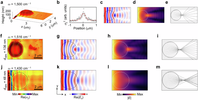
a Near-field image (real part) of a polaritonic Lunrburg lens, Re(σ2), at the frequency (ω) of 1500 cm−1, overlapped on its three-dimensional topography, where the thickness of the hBN slab (dhBN) is 89 nm. b Line scan signals along the focal spot and corresponding Gauss fitting. c Simulated field distribution in the x−y plane, denoted by the real part of the electric field in the z direction, Re(Ez). d Corresponding magnitude of the simulated electric field (|E | ). e Ray-tracing result. Experimental (f) and simulated results (g–i) for another polaritonic Luneburg lens with a larger size. j–m Same as (f–i) but for a polaritonic lens with a gentler index distribution than that of a Luneburg lens. Green and grey curves indicate the concave interference patterns resulting from edge-launched and edge-reflected tip-launched polaritons, respectively.
The dimensions of the prepared PMMA caps can be conveniently adjusted by varying the size of the PMMA microsphere used in the fabrication process. Figure 4f presents a polaritonic Luneburg lens fabricated from a larger PMMA microsphere, yielding a larger focal spot with a resolution of 1.04 μm (λ0/6), consistent with simulations in Fig. 4g−i. This decrease in resolution is due to the larger λp supported by the thicker hBN slab with dhBN = 136 nm, indicating the essential role of polariton wavelength in the performance of polaritonic Luneburg lenses (Supplementary Note 2). The resolution can be improved by reducing hBN thicknesses or shifting frequencies, as demonstrated by the simulation results in Supplementary Fig. 7, where a resolution of λ0/39 is achieved with a 30 nm-thick hBN slab at 1510 cm−1.
Beyond polaritonic Luneburg lenses with pre-defined neff distributions, other polaritonic lenses with gradient neff can be realised by modifying the PMMA geometry or adjusting the operating frequency—two approaches that are functionally equivalent in shaping neff. As demonstrated in Fig. 4j−l, the concave interference patterns observed within the PMMA cap exhibit reduced curvature compared to those in Luneburg lenses due to a gentler neff gradient. Additional interference fringes (grey curves) appear in the near-field image, exhibiting a periodicity reduced to half that predicted by simulations. These features are attributed to edge-reflected polaritons launched by the tip (Supplementary Fig. 8). The focal spot in this lens is less distinct, which is caused by dispersive electric fields, as corroborated by the ray-tracing result in Fig. 4m. By contrast, a steeper neff gradient promotes rapid convergence, shifting the focal spot beneath the PMMA cap and thereby limiting its detectability in near-field measurements. To ensure clear identification of the focal spot, we deliberately choose a slightly lower neff than the ideal value in Fig. 4a. A comprehensive frequency-dependent evolution of the focusing behaviour is provided in Supplementary Fig. 9.
Our strategy is not limited to PMMA; other polymers, as well as organic or inorganic materials with predefined geometries and appropriate thermodynamic properties, could also be employed to serve as dielectric components and create gradient polaritonic lenses via our lithography-free approach. As a proof-of-concept demonstration, we prepared a gradient polaritonic lens using a polystyrene (PS) microsphere, following a similar procedure in Fig. 3a. Because of the slightly higher dielectric permittivity of PS (εPS ≈ 2.4), the required PS geometry for a polaritonic Luneburg lens varies from that of PMMA. The theoretical geometry and refractive index are depicted by orange curves in Fig. 5a,b, which are satisfied excellently by the PS microstructure (blue curve) obtained by our lithography-free method and fitted by our spherical cap model. The near-field image of the fabricated device is shown in Fig. 5c, where the concave wavefronts over the PS region indicate gradually focused polaritons, culminating in a focal spot with a resolution of 0.52 μm (λ0/13). These features are qualitatively reproduced by numerical simulations (Fig. 5d, e) and ray-tracing results (Fig. 5f). Additional PS-based lenses and corresponding near-field images are provided in Supplementary Fig. 10, demonstrating the reproducibility of our approach.
Fig. 5: Lithography-free strategy for versatile polaritonic lenses.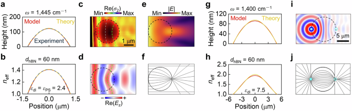
a Cross-sectional height profile of the prepared polystyrene (PS) cap (blue), aligning well with the spherical cap model (red) and theoretical Luneburg lens geometry (orange) at the frequency (ω) of 1445 cm−1. The thickness of the hBN slab (dhBN) is 60 nm. b Corresponding distribution of effective refractive indices (neff). c Near-field image (real part) of a polaritonic Lunrburg lens, Re(σ2). Numerical simulation (d, e) and ray-tracing results (f). Cross-sectional height profile (g) and index distribution (h) of a proposed spherical cap atop an hBN slab, agreeing well with the required theoretical Maxwell fisheye lens. The permittivity of the dielectric layer (εdl) is set to 7.5. i Field distribution over the spherical cap excited by a z-polarised dipole (cyan dot), where a mirrored focal spot (cyan circle) at the opposite position of the lens rim is formed. (j) Ray-tracing result for the polaritonic Maxwell fisheye lens.