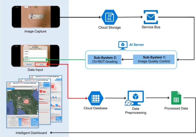
This section delves into the artificial intelligence (AI) components integral to the OV-RDT platform. We describe the dataset used for training and evaluation, while describing two main AI subsystems—1) image quality control and 2) OV-RDT grading. We also explain the evaluation metrics and the experimental design employed to validate the performance of these AI subsystems. Finally, the results, discussion, and effectiveness of the AI implications in improving diagnostic accuracy are presented.
Dataset
In this experiment, we utilized a dataset comprising 8,624 OV Rapid Test Kit images, all meticulously collected and annotated by experts to ensure high data quality. The dataset was divided based on a train-test split criterion: 6,900 images were allocated for training the model, while the remaining 1,724 images were reserved for testing. This approach ensured that the model’s performance could be evaluated on a separate, unseen set of images, providing a reliable measure of its generalization capability and accuracy in real-world scenarios. The dataset was collected during the Cholangiocarcinoma Research Institute (CARI) outreach between 18 February and 1 June, 2024. To ensure experimental integrity and prevent data leakage, this train-test split was performed once at the beginning of the study and maintained consistently across all experiments. The test set of 1,724 images was never exposed to any model during training or hyperparameter optimization phases. We named it the OV-RDT classification dataset which only contains good quality strip images. The demographic distribution of the dataset is summarized in Table 1.
Additionally, we collected 100 images of OV Rapid Test Kits labelled as failed capture images during the application’s image capture process. These images were specifically used to evaluate the image quality control subsystem. We also randomly selected 100 successful capture images from the existing OV-RDT Classification dataset. This combination created a balanced dataset, allowing us to thoroughly assess the model’s performance in estimating image quality across various capture conditions. In addition to the main classification dataset, we collected a separate dataset for training the image quality control system. This comprised 574 OV Rapid Test Kit images captured through dedicated data collection sessions designed to include various capture conditions, positioning errors, and lighting scenarios. These images were systematically annotated with bounding boxes for the YOLOv5m object detection model training, ensuring a well-balanced dataset for developing robust quality control capabilities.
Table 1 Demographic characteristics of the participants found in the OV-RDT classification dataset.AI sub-system 1: image quality control
This AI-based module’s advantage lies in its ability to locate the OV Rapid Test Kit within images collected from the OV-RDT mobile application. The YOLOv5m model was utilized as the baseline architecture for detecting the OV Rapid Test Kit in images. As a medium-sized model within the YOLOv5 family, YOLOv5m is well-regarded for real-time object detection tasks with a good balance of accuracy and speed. For model training, we utilized a dedicated dataset of 574 annotated OV Rapid Test Kit images collected through controlled data collection sessions using our OV-RDT mobile application (both Android and iOS versions) during the early development phase (January-February 2024). This dataset was specifically designed to be well-balanced for machine learning model development, separate from the main OV-RDT classification dataset, ensuring representation of various capture conditions and positioning scenarios. From these 574 images, 479 were used for training, while the remaining 95 images were allocated for validation. All experiments were conducted on a workstation equipped with two NVIDIA GeForce RTX 2080 Ti GPUs. It is important to note that the dataset used for training the YOLOv5m image quality control model (574 images) was completely separate from the OV-RDT grading dataset (8,624 images), ensuring no data leakage between these two subsystems.
The system integrates a verification step known as the quality module, which is described in Algorithm 1. This module verifies the correctness of the test kit’s positioning within the camera template by checking the location of the detected bounding box and comparing it with predefined spatial constraints. If the detected box deviates from the expected location by more than a specified margin, the system prompts the user to retake the image.
The YOLOv5m model was fine-tuned with a specific set of hyperparameters designed to optimize detection accuracy for the OV-RDT domain. The training configuration is detailed as follows:
-
Learning Rate: We utilized an initial learning rate of 0.001 with OneCycleLR scheduling, decreasing to 0.0001 (\(lr0 \times lrf = 0.001 \times 0.1\)) over 400 epochs. A warmup period of 3 epochs was applied with a warmup bias learning rate of 0.1.
-
Batch Normalization: Applied across all layers with a momentum coefficient of 0.937.
-
Optimizer: The model was optimized using Stochastic Gradient Descent (SGD) with momentum = 0.937 and weight decay = 0.0005, including an initial warmup momentum of 0.8.
-
Batch Size: Training was performed with a batch size of 16 using input images resized to 640\(\times\)640 pixels.
-
Augmentation: Various data augmentation techniques were used, including mosaic augmentation (probability = 1.0), random scale transformations (±0.5), translation adjustments (±0.1), and HSV color space modifications (hue ±0.015, saturation ±0.7, value ±0.4).
-
Loss Function: A composite loss function was employed, comprising box loss (gain = 0.05), classification loss (gain = 0.5), and objectness loss (gain = 1.0), with an IoU training threshold of 0.20 and anchor-multiple threshold of 4.0.
This training setup enabled robust and consistent detection of OV test kits across a wide variety of image capture conditions, laying the foundation for reliable downstream grading and classification tasks in the OV-RDT platform.
Algorithm 1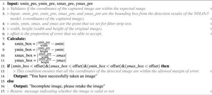
OV-RDT strip image quality control algorithm.
Algorithm 1 requires four parameters: \(xmin\_pre\), \(ymin\_pre\), \(xmax\_pre\) and \(ymax\_pre\) (bounding box). These four parameters represent the bounding box of the detected OV-Rapid test kit. The margin of the bounding box is compared to that of the predefined bounding box characterised by \(xmin = 0.271307\), \(ymin = 0.389985\), \(xmax = 0.780217\) and \(ymax = 0.589000\). Then, we compute the margin error between the detected bounding box and the predefined one. Images are considered successfully capturedif the margin error is less than or equal to the offset value (\(offset = 0.03\)); otherwise, it is classified as a failed capture. The combination of standardized image capture through the camera template and YOLOv5m-based detection creates a robust quality control system. Images with poor quality characteristics such as blur or inadequate lighting naturally fail the detection process, as the YOLO model’s confidence drops below the acceptance threshold in these cases.
Fig. 2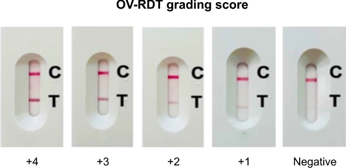
The standard OV-RDT color chart for the score based on the band intensity from \(+1\) to \(+4\) was constructed using Opisthorchis viverrini crude antigen diluted in clean urine. The color intensity at T was expressed as \(+4\) for the highest intensity and \(+1\) for the lowest intensity, implying lover of infection.
AI sub-system 2: OV-RDT grading
We employed artificial intelligence to predict OV-RDT grading scores ranging from 0 to +4, as illustrated in Fig. 2. The grading scores correspond to two diagnostic statuses: Negative (score 0) and Positive (scores +1, +2, +3, or +4). Our experimental dataset comprised 8,624 expert-annotated images of OV Rapid Test Kits, divided into 6,900 training images and 1,724 testing images. All images underwent quality control using YOLOv5m before model training. We evaluated multiple machine learning approaches for both multi-class grading (five levels: 0, +1, +2, +3, +4) and binary classification (Negative vs. Positive). EfficientNet-B5 was selected as the primary deep learning architecture due to its optimal balance between model size and accuracy, making it particularly suitable for mobile deployment. We benchmarked this against other proven architectures, including ResNet5015 and MobileNetV226 for both classification and regression tasks, providing insights into performance trade-offs across different neural network architectures for OV-RDT interpretation.
Additionally, we implemented traditional machine learning models—Random Forest27 and Support Vector Machine (SVM)28 for multi-class classification. These models utilised feature vectors derived from red (R), green (G), and blue (B) colour values extracted from the test result area, following the methodology of DentShadeAI29. We specifically focused on the green channel, which provided optimal contrast for T-band detection as shown in Fig. 3. Both traditional models were trained using the Scikit-Learn package30 with five-fold cross-validation for hyperparameter optimisation. The five-fold cross-validation for Random Forest and SVM models was conducted exclusively within the training set of 6,900 images, with the test set of 1,724 images held out for final evaluation only.
The EfficientNet-B5 training was conducted using TensorFlow with pre-trained ImageNet weights and executed on a workstation equipped with dual NVIDIA GeForce RTX 2080 Ti GPUs. A two-phase transfer learning strategy was employed: in the first phase, all convolutional layers were frozen and only the classification head was trained for 200 epochs. In the second phase, layers from Block 5 onward were unfrozen and fine-tuned for an additional 200 epochs, allowing the model to adapt to OV-RDT-specific features. A batch size of 16 was used throughout, with RMSProp selected as the optimizer, an initial learning rate of \(2 \times 10^{-5}\), and categorical cross-entropy as the loss function (mean squared error was used in regression experiments). To enhance model generalization and mitigate overfitting, a variety of data augmentation techniques were applied, including random rotation (\(\pm 10^\circ\)), zoom (\(\pm 10\%\)), brightness and contrast shifts (\(\pm 20\%\)), and random cropping and resizing. Horizontal flipping was excluded due to the direction-sensitive layout of the test kits. Regularization techniques included L2 weight decay (\(1\times 10^{-5}\)), dropout (rate = 0.3), early stopping (patience = 15 epochs), and adaptive learning rate reduction via ReduceLROnPlateau (factor = 0.5 after 5 stagnant epochs). On average, training required approximately 12 hours per model. The final model size was approximately 119 MB, and inference time was around 60 ms per image, supporting real-time performance on mobile devices. This training pipeline enabled EfficientNet-B5 to deliver high performance across both fine-grained multi-class grading and binary OV infection classification in real-world screening scenarios. While color normalization and stain standardization techniques have shown promise in medical image analysis, we opted to rely on the robustness of pre-trained models and our standardized image capture protocol for this initial implementation. Future work will investigate preprocessing methods specifically tailored to RDT strip analysis to potentially enhance grading accuracy, particularly for cases with subtle T-band intensity differences.
For model interpretability, we implemented GradCAM using the TensorFlow GradCAM library, extracting activation maps from the final convolutional layer (\(top\_conv\)) of our fine-tuned EfficientNet-B5 model. The gradients were computed with respect to the predicted class score, and the resulting heatmaps were resized to match the input image dimensions (224×224) using bilinear interpolation.
Fig. 3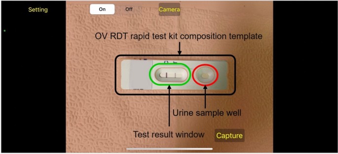
An example image when placing the OV-Rapid test kit within a camera template to ensure image quality on both positioning and distance between the strip and the camera.
Evaluation metrics and experimental design
We used a confusion matrix to evaluate the performance of the OV infection classification model. The evaluation was conducted on a test set comprising 1, 724 images, all of which had passed the image quality control step. The confusion matrix is a standard tool for analyzing classification models, providing a detailed breakdown of prediction outcomes by comparing predicted labels with ground-truth annotations. It reports results in terms of four key categories: true positives (TP), where positive cases are correctly identified; true negatives (TN), where negative cases are correctly classified; false positives (FP), where negative cases are incorrectly predicted as positive; and false negatives (FN), where positive cases are missed by the model. This categorization offers insight into not only overall model performance but also the types of errors that occur.
Based on the confusion matrix, we computed four performance metrics: accuracy, precision, recall, and F1-score. Accuracy represents the proportion of correct predictions among all predictions made. Precision measures the proportion of true positives among all predicted positives, reflecting the model’s ability to avoid false alarms. Recall (or sensitivity) indicates the model’s ability to detect actual positive cases, which is particularly critical in medical screening applications where missing a positive case can have serious consequences. The F1-score combines precision and recall into a single metric, providing a balanced measure of the model’s performance, especially in cases where the class distribution is imbalanced. Together, these metrics offer a comprehensive evaluation of the model’s reliability in real-world OV-RDT classification scenarios.
To evaluate the performance of the image quality control module, we used a dataset of 200 OV-RDT images, comprising 100 successful captures and 100 failed ones, as labeled by domain experts. The model’s performance was measured using accuracy, precision, and recall. To further analyze its behavior, we categorized the results into four outcome types. True positive cases refer to instances where the test kit was properly placed within the camera frame and was correctly detected. These images typically featured good lighting, centered alignment, and correct orientation. True negative cases occurred when the test kit was improperly positioned, for example skewed, off-center, or blurred, and the model correctly rejected them. False positives describe cases where the model accepted an image that was not properly positioned, often due to slight misalignment or uneven lighting. False negatives occurred when the test kit was placed correctly but the model failed to detect it, usually because of glare, background interference, or poor contrast. This classification provides insight into the model’s strengths and the types of errors that can arise under real-world image capture conditions.
To establish a robust statistical framework for classification evaluation, we systematically partitioned the test dataset into 30 non-overlapping subsets (n\(\approx\)60 samples per subset) using randomized sampling without replacement. Model performance was quantified across four complementary metrics: accuracy, precision, recall, and F1-score. For each metric, we calculated both the sample mean and standard deviation across all subsets. In accordance with the central limit theorem, we verified that the sampling distributions of performance metrics approximated normal distributions. Homogeneity of variance across the eight methods was confirmed via Levene’s test prior to conducting inferential analyses. We then employed one-way ANOVA to test the null hypothesis of equal mean performance across methods. Where the ANOVA null hypothesis was rejected (p
To assess the clinical implications of model performance, we analyzed the confusion matrix to identify patterns in misclassification, particularly focusing on clinically significant errors (e.g., false negatives in binary classification or misclassification by more than one grade level in multi-class grading). The moderate Kappa score (0.55) for multi-class grading reflects the subjective nature of visual intensity assessment, a known challenge in immunochromatographic test interpretation that our platform addresses through human oversight and adaptive threshold management.
Results and discussion
The EfficientNet-B5 model for image quality control exhibited outstanding performance in assessing image quality. The model achieved accuracy, precision, and recall scores of 98.00%, 95.00%, and 100.00%, respectively, indicating high reliability. An accuracy of 98.00% reveals that the model accurately classified the vast majority of images, while a precision of 95.00% indicates that nearly all images predicted to be of high quality were indeed high quality. The perfect recall score of 100.00% also underscores that the model successfully identified all high-quality images, capturing all relevant cases. The high performance of our quality control approach (98% accuracy) validates that the YOLOv5m model, when combined with our fixed capture template and spatial verification algorithm, provides sufficient quality assurance for downstream classification tasks. This approach effectively filters out images with quality issues including blur, poor lighting, and improper positioning without requiring additional pre-processing steps. The effectiveness of the model is further illustrated in Fig. 4, where examples of true positive, true negative, and false positive images are presented. These examples highlight how the model distinguishes between correctly identified high-quality images (true positives), correctly identified low-quality images (true negatives), and cases where the model mistakenly classified low-quality images as high-quality (false positives). This high level of performance makes the EfficientNet-B5 model an excellent choice for practical applications in automated image quality assessment.
Fig. 4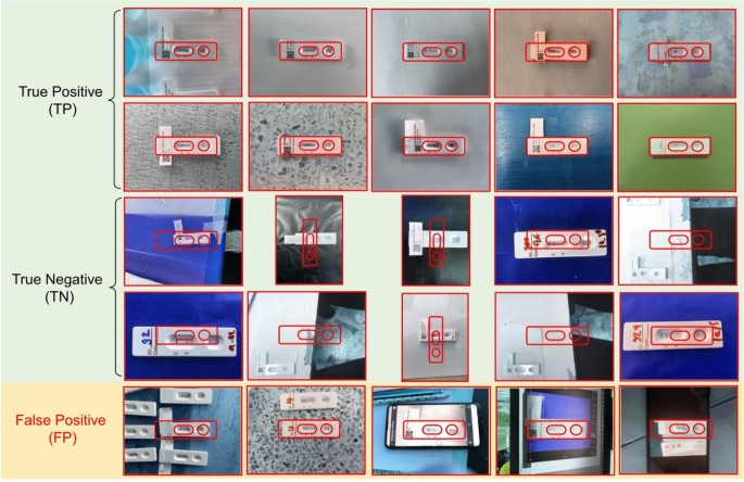
Examples of results from the OV-RDT strip image quality control algorithm: True Positive indicates the examples that the algorithm accurately classify as good quality images, True Negative indicates the examples that the algorithm accurately classify as poor quality images, and False Positive indicates the examples that the algorithm mis-classify as good quality images.
Fig. 5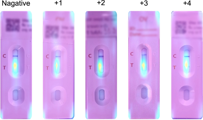
GradCAM visualization showing model attention patterns for OV-RDT grading. Representative heatmaps for each infection grade (0 to +4) demonstrate that the model correctly focuses on the T-band region, with activation intensity correlating with infection severity. Warmer colors (red/yellow) indicate regions of higher importance for the model’s decision.
Table 2 Comparison of different machine learning models on the performance in estimation OV infectious level grading. The best performance and the next best performance are indicated in bold and italic respectively. \(\circ\) represents a classification model and \(\triangle\) represents a regression model. The proposed models that outperform the most performant baseline, ResNet50 \(\triangle\) (\(p ) are marked with \(*\).
Table 2 presents the experimental results for classification tasks. The sample mean plus/minus standard deviation across eight methods was computed for each performance metric. Since the null hypothesis of the ANOVA test was rejected, the Multiple Comparisons of Means – Tukey HSD analysis was conducted to differentiate the performance across eight state-of-the-art methods statistically. EffNet-B5-based model for regression demonstrated clear statistical superiority over most competing models (p
Model interpretability analysis
To enhance the transparency and trustworthiness of our AI system, we implemented Gradient-weighted Class Activation Mapping (GradCAM) to visualize the regions of OV-RDT images that most influence the model’s grading decisions. GradCAM generates visual explanations by examining the gradients flowing into the final convolutional layer of our EfficientNet-B5 model, highlighting the discriminative regions used for classification.
We applied GradCAM analysis to a representative subset of 100 test images across all five grading levels. The resulting heatmaps were overlaid on the original OV-RDT images to identify which spatial regions contributed most significantly to the model’s predictions. As shown in Fig. 5, the GradCAM visualizations demonstrate that our model correctly focuses on the T-band (test line) region when determining infection grades. The intensity of activation in the T-band area progressively increases from grade 0 (negative) through grade +4, corresponding to the visual intensity of the test line itself.
This analysis provides important validation that our model has learned to identify clinically relevant features rather than relying on spurious correlations or image artifacts. The concentrated attention on the T-band region aligns with expert diagnostic practices, where the color intensity of this specific area directly indicates the level of OV antigen present in the urine sample.