Flocculation dynamics and knowledge embedding
There is a quantitative relationship between flocculants and granules, In flocculation dynamics, the forces driving particle collisions come from two sources: (1) particle collision and aggregation caused by Brownian motion is called perikinetic flocculation (Text S1); (2) particle collision and aggregation caused by fluid motion from hydraulic or mechanical agitation is called orthokinetic flocculation (Text S2). The detailed process is described in Text S1, Text S2. Although perikinetic flocculation itself is not affected by particle size, as particle size increases, the effect of Brownian motion diminishes. To further promote collision and aggregation of larger particles, orthokinetic flocculation is also required. For real water bodies, where perikinetic flocculant and orthokinetic flocculant coexist, the ratio of different collision types is uncertain. In addition, the particle size (d) and collision efficiency (\(\eta\)) also vary with changes in water quality (Text S1, Text S2). Therefore, the accurate dosing amount cannot be described by a quantitative formula, but is more suitable for learning the nonlinear relationship through ML and the types of data collected need to include water quality indicators for different sections of the full process.
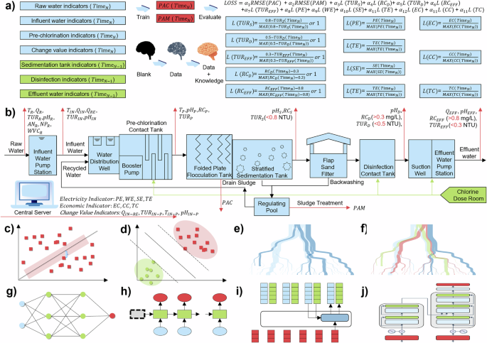
How to embed environmental knowledge into the model and thus increase the interpretability of the model is key to the research. The study also considered the economic benefits and energy expenditure. The logical chain of the flocculation process is, addition of flocculant ➝ change in kinetic characteristics ➝ particle flocculation ➝ change in water quality of the flocculation section ➝ change in subsequent water quality ➝ change in water quality of the effluent, and the related economic indicators. Thus, 7 economically relevant indicators (4 electricity indicators and 3 economic indicators recorded by the central server were used as constraints rather than independent variables to optimize the model parameters for use in the training phase, while in the inference and application phases these indicators have been embedded as knowledge in the model (Eq.1, Fig. 1a). Similarly, the metrics before the flocculation segment at timen and after the flocculation segment at timen-1 are used as independent variables, and the metrics after the flocculation segment at timen are used as constraints. The change value features are calculated in real time by the central server along with the results of online monitoring.
$$\begin{array}{c}\begin{array}{cc}{Train}: & {PAC}={ML}\left({WIBC}\right)* {MLP}\end{array}\\ {MLP}\leftarrow {a}_{1}{Loss}({WIBC})+{a}_{2}{Loss}({WTIAC})+{a}_{3}{Loss}({PTIAC})+{a}_{4}{Loss}({ETIAC})\\ \begin{array}{cc}{Test}: & {PAC}={ML}\left({{WIBC}}_{{Test}}\right)* {MLP}\end{array}\end{array}$$
(1)
\({ML}\) is different machine learning models
\({MLP}\) is different machine learning model parameters
\({WIBC}\) is water quality indicators before coagulation
\({WTIAC}\) is water quality threshold indicators after coagulation
\({PTIAC}\) is power threshold indicators after coagulation
\({ETIAC}\) is economic threshold indicators after coagulation
With the distinction between independent variables and constraints, and then the knowledge of environmental science embedded in the model training process, it is possible to clearly set the problem framework, optimize the calculation process, and improve the efficiency and accuracy of the model. As for the threshold control after the flocculation section, after the disinfection section, and before leaving the plant, the evaluation standard is the closer to the threshold, the better, rather than the lower and lower water quality, the better. Because of the need for water quality, economic costs, and environmental benefits of a comprehensive balance. Finally, an interpretable analysis of the constructed model is performed along with application validation.
Treatment process and data collection
The DWTP from which the data was obtained is located in Guangzhou, China. The design water supply capacity is 800,000 tons per day, the actual water supply capacity is 450,000 tons per day, and the total construction land area is about 180,000 m2. The plant adopts the chlorine disinfection process of pre-chlorination, 3 sodium hypochlorite at the water intake, the disinfection contact pool, and the water delivery pumping station before (Fig. 1a, b). Coagulation chemicals used PAC (Polymerized Aluminum Chloride), the main parameters of PAC are shown in Text S3. China’s current water quality standards for water leaving the plant is GB5749-2022, the water plant to implement more stringent control standards, specifically after the sedimentation tank controls turbidity less than 0.8NTU, after the disinfection tank controls turbidity less than 0.5NTU, the residual chlorine is greater than 0.3 mg/L, the effluent control turbidity is less than 0.3NTU, the residual chlorine is greater than 0.8 mg/L.
To improve the feasibility of the subsequent design, the study selected 38 indicators that can be measured online at most water plants (Fig. 1a). These included 7 raw water indicators,5 influent water indicators, 4 pre-chlorination indicators, 3 sedimentation tank indicators, 3 disinfection indicators, 4 effluent water indicators, 4 electricity indicators and 3 economic indicators recorded by central server, 4 change value indicators by independently designing and calculating, as well as the dosage of PAC (Table S1). The study provided instrument conFig.urations, installation locations, quantities and categories (Table S2). The dataset is divided with a ratio of 8 to 2 between the training set and the test set.
ML principles
For the feasibility of the ML approach, eight ML algorithms were selected for the study29,30,31 (Text S4). It includes Ridge Regression (RIDGE), Support Vector Regression (SVR), Random Forest (RF), Extreme Gradient Boosting (XG), Deep Neural Networks (DNN), Recurrent Neural Networks (RNN), Long Short-Term Memory Networks (LSTM), and Transformer (TF). RIDGE is the baseline model.
RIDGE is a method to improve the stability and predictive power of linear regression by regularizing the penalty term (Fig. 1c). SVR fits linear and nonlinear data via support vector machines (Fig. 1d)32,33. RF is an ensemble learning based on bagging, the subtrees are independent and do not affect each other (Fig. 1e)34,35,36. XG is also an ensemble learning, but it’s based on boosting and the subtrees are dependent on each other (Fig. 1f)37,38,39. DNN consists of multiple layers of neurons and are the simplest deep learning networks (Fig. 1g)40,41,42. RNN captures time dependence in temporal data through cyclic connectivity, but may face gradient vanishing during training (Fig. 1h)43. LSTM controls the flow of information by introducing a gating mechanism that allows the network to selectively retain important information and forget irrelevant information (Fig. 1i)44,45,46. TF captures global information through a self-attention mechanism that allows each input element to be computed in association with all other elements in the sequence (Fig. 1j)47,48,49.
Model interpretability
Shapley Additive Explanations (SHAP) is an explanatory method based on game theory for measuring the contribution of each feature to the prediction results of a ML model50,51. It draws on the concept of Shapley value to derive the contribution value of each feature by calculating the marginal contribution of the features to the prediction in different combinations52,53.The advantage of SHAP is that it provides transparency in model prediction, reveals the specific impact of features on the results, and helps to understand the decision-making process of complex models40,54. During model development, SHAP can help developers identify potential errors or unfair factors and avoid model bias.SHAP is used to understand and validate the ML dosing model in this study.
Subtree depths in Random Forest (RF) can increase the interpretation and understanding of the model. Subtree depth directly affects model complexity, generalization ability, and computational efficiency: trees with greater depth may capture complex patterns but are prone to overfitting, while trees with less depth are simpler and easier to interpret. By adjusting the depth, model performance and interpretability can be balanced to help diagnose overfitting or underfitting problems. In addition, subtree depth affects feature importance analysis and the transparency of decision paths, making the model decision process easier to understand and communicate.
Application feasibility verification
DWTP adopts folded plate flocculation tanks, and the flocculation area is divided into 2 blocks, a total of 8 groups, the length, width and height of each group are 13.75 m, 14.40 m and 7.1 m respectively. Each group of flocculation tank is divided into 3 rows, 2 columns and 6 areas, and the total number of folded plates is 38 blocks. The model constructed during the validation was scaled down 25 times, and the length, width and height of one group were 55 cm, 57.6 cm and 28.4 cm respectively. The designed hydraulic retention time of the flocculation area was 15.1 min, and the designed hydraulic retention time of the sedimentation area was 102 min.
The validation will take place from February 4, 2025 to February 13, 2025, a total of 10 days. There were four sampling time points, 10:00, 12:00, 14:00, and 16:00 daily.The validation was done by directly taking the water before coagulation, calculating the dosing scheme for the original logic of the water plant and the ML-driven dosing scheme, respectively, and mixing the water and the pharmaceuticals through the pump. The water was then fed into two identical downsized flocculation reactors and the coagulated water was left to stand for 102 min to test the indicators. Considering the differences between the reactors and the real water plant, the indicators of the real water plant during the reactor validation were also collected online and used for comparison. All tanks appear in pairs, so separate controls are performed to verify the migratability of the method.
Technical economic analysis (TEA) assesses the economic feasibility, benefits and risks of technologies through quantitative and qualitative analyses, thus providing a scientific basis for decision-making. This study mainly considers the cost of chemical consumption, which mainly includes flocculant (PAC), disinfectant (sodium hypochlorite) and other agents. Other chemicals mainly refer to hydrochloric acid and sodium hydroxide used in backwashing to adjust the pH.
Monte Carlo simulation is an effective numerical method for addressing uncertainty issues, offering advantages such as simplicity of implementation, strong reproducibility, and applicability to perturbation analysis of complex systems. This study introduces this method to assess the robustness of the model under data missing conditions. Specifically, for each specified missing proportion, a corresponding proportion of feature values are randomly selected from the original input data and set to 0 to simulate real-world monitoring anomalies such as sensor failures, communication interruptions, or missing data records. Subsequently, the model is run 100 times based on the disturbed data, and the error from each simulation is recorded. Through statistical analysis of the results from multiple simulations, the performance fluctuations and stability of the model under different missing data ratios can be quantified.