Study design and setting
The Mayo Clinic institutional review board approved this study, which was conducted in accordance with the relevant guidelines (e.g., TRIPOD + AI (Transparent Reporting of a Multivariable Prediction Model for Individual Prognosis Or Diagnosis + Artificial Intelligence)) and regulations28. Only patients who authorized the use of their health records for research were included in the analysis, and the need to obtain informed consent was waived by the Mayo Clinic institutional review board. We retrospectively searched our institution’s electronic health record system (Epic Corporation) to identify patients seen in seen at EDs on any of Mayo Clinic’s 3 campuses (Rochester, Minnesota; Jacksonville, Florida; and Phoenix, Arizona) and the Mayo Clinic Health System (various locations in Minnesota, Wisconsin, and Iowa)EDs at [blinded institution name, geographic location] from January 1, 2017, through December 31, 2021.
Patients
We created a data set of ED encounters that initially included all ED patients who had a urinalysis or a urine culture result. No age restrictions were applied. For inclusion in the study, records needed to have documentation of ED arrival and departure (dates and times) and ED encounter diagnoses listed. The urinalysis and urine cultures had to be ordered 4 h before to 8 h after the ED arrival. For urine cultures, the collection date and time had to be recorded, and the results documented within 10 days after sample collection. All encounters included documented event start and end dates and times, admit and discharge dates and times, encounter admit and discharge dates, and diagnosis dates (as per the terminology used in the electronic health record). We included only encounters that reported values for all the following urine studies: red blood cells, white blood cells, nitrite, bilirubin, leukocyte esterase, glucose, specific gravity, protein, pH, ketone, and urobilinogen.
Variables and primary outcomes
Each patient had a unique clinic number that enabled analysis of data over time, and each encounter in the data set received a unique identifier. From each patient’s health record, we extracted data regarding demographic characteristics, medical history (including past ED urine culture results, allergies, and reproductive health information), and social history. We also collected temperature, laboratory and radiologic studies, diagnoses before the urine culture result was known, medications ordered before and during the ED encounter, hospital admission and disposition, genitourinary nursing procedures and flowsheets, and nurse-assessed fall risk. When relevant data were available, we calculated established estimators of inflammation (e.g., urinary inflammatory index, systemic immune-inflammation index, neutrophil-lymphocyte ratio, platelet-lymphocyte ratio), as well as ratios and mathematical formulas, based on laboratory test results, that we developed (Supplement 1)29.
We chose three primary outcomes for urine cultures:
-
(1)
No microbial growth vs. any microbial growth (including mixed flora).
-
(2)
≥10,000 CFU/mL for ≥1 bacterial species vs.
-
(3)
≥100,000 CFU/mL for ≥1 bacterial species vs.
For our secondary analyses, we used extreme gradient boosting (XGBoost) to determine how well the model predicted likely false-positive UTIs, in which a UTI was diagnosed before urine culture results were known and no growth was reported for the urine culture. XGBoost is a machine learning approach that combines prediction models to create a more robust model. We also examined how well the model predicted potentially true-positive UTIs, in which a UTI was diagnosed before urine culture results were known and cultures showed ≥100,000 CFU/mL for ≥1 bacterial species.
Diagnoses
We identified encounter diagnoses, including ED and any inpatient diagnoses, by searching the data set for International Classification of Disease, Tenth Revision codes and text strings (Supplement 2). We included diagnoses in our algorithms only if the ED discharge and departure date and time, event end date and time, encounter discharge date, and diagnosis date were all before the date and time that urine culture results were known.
Statistical analysis
Each outcome was binarized to 1 for yes and 0 for no. If a particular diagnosis was not made during the encounter, then it was coded as no. Likewise, if the urine culture result was known before the date and time of ED discharge and departure, event end date and time, encounter discharge date, or diagnosis date, the diagnosis outcome also was coded as no. Missing data were accounted for by labeling it as not available for categorical data and using the median value for continuous variables. All available data were considered in the analysis (e.g., average microbial growth for all available urine cultures). Depending on the algorithm used, the same data could be entered as either a continuous or categorical variable. For example, urine leukocyte esterase data could be input as a range (e.g., values from 0 to 4), as qualitative descriptors (e.g., none, trace, small, moderate, or large), or as a binary variable (present vs. absent). Categorical outcomes were one-hot encoded.
Data were characterized as either features or target variables. The data were then randomly split into training and testing sets, with 20% in the testing set. Synthetic minority oversampling was applied to create synthetic samples for the minority class (to resolve class imbalance). A standard scalar was applied, and a series of models were then fitted: logistic regression classifier, k-nearest neighbors classifier, random forest classifier, XGBoost classifier, and a deep neural network classifier. Default hyperparameters were applied for each model. The XGBoost model was configured with default settings and early stopping rounds with a logloss evaluation metric. The neural network was configured with three dense layers with 128 neurons (relu activation), 64 neurons (relu activation), and 1 neuron (sigmoid activation), with dropout layers between layers 1 and 2 and between layers 2 and 3 to prevent overfitting. Early stopping was applied, and the model was compiled with an adam optimizer with binary_cross entropy as the loss function.
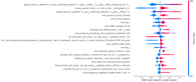
The reported performance metrics included accuracy, area under the receiver operating characteristic curve (AUROC), class-positive precision, recall, and F1 score. The model with the best performance was selected for additional analysis. Shapley additive explanation (SHAP) values were calculated on the test set to explain the model’s output. The 25 variables with the highest SHAP values were selected for additional analysis, and models were rerun by using a data set with only those 25 variables.