Actinomycin D is used as an antineoplastic antibiotic that intercalates into DNA, thereby preventing RNA synthesis. It is primarily employed to treat gestational trophoblastic neoplasia, Wilms tumor, and rhabdomyosarcoma. It interferes with transcription by binding to the DNA double helix and blocking RNA polymerase mobility. It is administered intravenously, usually as part of combination chemotherapy. Common adverse effects include bone marrow suppression, vomiting, alopecia, and nausea20. Due to its high toxicity, dosing must be precise and closely monitored. Resistance may occur through increased efflux or alterations in drug targets. While its cell cycle-arresting capabilities contribute to its effectiveness, it must be used with caution, as it can cause tissue necrosis if extravasation occurs during administration.
Anastrozole is a nonsteroidal aromatase inhibitor primarily used in postmenopausal women to treat hormone receptor-positive breast cancer. It suppresses the action of the enzyme aromatase, which converts androgens to estrogens, thereby lowering estrogen levels that promote certain breast cancers. Anastrozole is administered orally, typically once daily. Common side effects include hot flashes, joint pain, weakness, and decreased bone density. Unlike tamoxifen, it does not increase the risk of uterine cancer or thrombosis21. It is commonly used as adjuvant therapy following surgery and can also be used in metastatic disease. Anastrozole is well tolerated and highly effective in significantly reducing the risk of recurrence. It is contraindicated in premenopausal women due to its estrogen-reducing mechanism.
Cabozantinib is a multi-kinase inhibitor that targets MET, VEGFR, RET, and other tumor-associated tyrosine kinases involved in tumor growth and angiogenesis. It is prescribed for advanced renal cell carcinoma, hepatocellular carcinoma, and medullary thyroid carcinoma. Administered orally, it inhibits pathways involved in cancer cell proliferation and angiogenesis. Adverse effects include diarrhea, fatigue, hypertension, hand-foot syndrome, and elevated liver enzyme levels22. It has shown efficacy in delaying disease progression and improving survival in various cancers. Dosage adjustments may be necessary due to toxicity. Since it interacts with CYP3A4 inhibitors and inducers, monitoring is required. Cabozantinib is a powerful targeted therapy that disrupts cancer cell survival and metastatic signaling pathways.
Cyclophosphamide is used in numerous cancers such as ovarian cancer, breast cancer, leukemias, and lymphomas as an alkylating agent. It cross-links DNA and results in cell cycle arrest and apoptosis in rapidly dividing cell populations. It is administered intravenously or orally as a prodrug activated in the liver23. The major toxicities are alopecia, bone marrow depression, hemorrhagic cystitis, nausea, and vomiting. Mesna is usually co-administered as a protector of the urinary bladder. It also finds application in the immunosuppressive treatment of autoimmune conditions such as lupus and multiple sclerosis. The oncological versatility of the drug arises from its wide range of activity against various cancers. Long-term treatment is risky and increases the likelihood of secondary cancers as well as infertility. Monitoring blood counts and hydration status is important to reduce toxicity and enhance drug efficacy.
Doxorubicin is an anthracycline antibiotic used in the treatment of several cancers, including breast cancer, lymphomas, and sarcomas. It intercalates DNA and causes DNA strand breaks through inhibition of topoisomerase II24. It also generates free radicals, contributing to its cellular toxicity. Doxorubicin is administered intravenously and possesses strong antitumor activity. The primary concern is cardiotoxicity, especially at cumulative doses, which is usually monitored via echocardiograms. Myelosuppression, vomiting, alopecia, and mucositis are other common adverse effects. Extravasation can cause tissue necrosis. Liposomal formulations are used to reduce cardiac risk. Doxorubicin remains a mainstay in chemotherapy regimens, although careful dosing and monitoring are essential to prevent severe adverse effects, such as irreversible myocardial damage.
Etoposide is a topoisomerase II inhibitor used in the treatment of small-cell lung carcinoma, testicular cancer, lymphomas, and leukemia. It inhibits DNA re-ligation during replication, leading to DNA strand breaks and cell death. Both intravenous and oral forms are available, and it is typically used in combination chemotherapy regimens. Myelosuppression, nausea, alopecia, and hypotension are frequent toxicities25. It is cell cycle-specific, acting mainly in the G2 and S phases. The efficacy of etoposide depends on dose and schedule, with drug efflux or enzyme changes occasionally leading to resistance. Close monitoring of blood counts and renal function is essential. Its inclusion in combination protocols makes it valuable in treating aggressive and resistant neoplasms.
Gemcitabine is a nucleoside analog used to treat pancreatic, lung, bladder, and breast cancers. Once incorporated into DNA, it blocks further DNA synthesis and induces apoptosis. It is administered intravenously as a prodrug, which is converted intracellularly into active metabolites26. Adverse effects include myelosuppression, influenza-like syndrome, rash, and mild gastrointestinal disturbances. It is usually combined with other chemotherapeutic agents for synergistic effects. The relatively low toxicity of gemcitabine allows for treatment of frail or elderly patients. It is widely used in treatment protocols due to its efficacy against solid tumors. Dosing regimens are adjusted based on the cancer type, and periodic monitoring of blood counts and liver function is necessary to ensure safety and efficacy.
Ibandronate is one of the bisphosphonates mainly used to treat and prevent osteoporosis and breast cancer metastases to bone. It inhibits bone resorption mediated by osteoclasts, resulting in increased bone mineral density. It is administered either orally or intravenously to decrease fractures and skeletal-related event risk. Gastrointestinal discomfort, flu-like syndrome, and osteonecrosis of the jaw are some of the adverse effects, though very rare27. Ibandronate can also be used to treat hypercalcemia of malignancy. It has a long bone tissue half-life, so dosing can be done once monthly. Proper administration (with water, while sitting or standing) is important to avoid esophageal irritation. The anti-resorptive action of ibandronate is useful in the management of both oncologic and metabolic bone diseases.
Ifosfamide is an alkylating agent most notably used in the treatment of testicular cancer, sarcomas, and lymphomas. It acts by inhibiting DNA replication, leading to the death of rapidly proliferating cancer cells. Administered intravenously, Ifosfamide is sometimes co-administered with other agents in chemotherapy to ensure greater efficacy28. Co-administration with mesna is necessary to prevent hemorrhagic cystitis, a toxicity affecting the bladder. Typical side effects include nausea, vomiting, bone marrow depression, and neurotoxicity. Hydration is also necessary during administration. Monitoring renal and hepatic function is required. Treatment with Ifosfamide is reserved for specifically selected patients based on the toxicity it can induce, especially central nervous system toxicity.
Letrozole is a nonsteroidal aromatase inhibitor most commonly used in postmenopausal women with hormone receptor-positive breast cancer. It acts by inhibiting the enzyme aromatase, which converts androgens into estrogens, thereby decreasing estrogen levels and inhibiting cancer progression29. It is administered orally, typically once a day. It is also used off-label to induce fertility in women with polycystic ovary syndrome (PCOS). Side effects can include hot flashes, tiredness, arthralgia, and an increased risk of osteoporosis due to reduced estrogen levels. Letrozole is highly valuable in both adjuvant and metastatic settings, particularly in hormone-sensitive breast cancer, and is recommended in current clinical guidelines. Long-term use may require bone density monitoring.
Pazopanib is an oral multi-target tyrosine kinase inhibitor (TKI) primarily used to manage advanced renal cancer and soft tissue sarcoma. It inhibits VEGFR, PDGFR, and c-KIT, thereby preventing angiogenesis and tumor growth. Pazopanib, taken once daily, is clinically beneficial in delaying disease progression30. Side effects include hypertension, diarrhea, fatigue, elevated liver enzymes, and hair color changes. Liver function tests should be monitored regularly due to the risk of hepatotoxicity. Pazopanib provides an alternative among available TKIs with an acceptable toxicity profile. However, it may interact with drugs metabolized by CYP3A4 and should be used cautiously in patients with hepatic or cardiovascular disease.
Regorafenib is an oral multi-target kinase inhibitor approved for metastatic colorectal cancer, gastrointestinal stromal tumors (GIST), and hepatocellular carcinoma. It targets VEGFR, PDGFR, FGFR, RAF, and several other kinases involved in tumor angiogenesis, oncogenesis, and the tumor microenvironment. Regorafenib is taken daily for three weeks in a four-week cycle and helps delay disease progression in patients who have failed prior therapies31. Side effects include hand-foot skin reaction, fatigue, diarrhea, hypertension, and hepatotoxicity. Blood pressure and liver function must be regularly monitored. Regorafenib s broad kinase inhibition results in numerous drug interactions. It is an essential option for patients with limited therapeutic alternatives and requires careful toxicity management.
Sorafenib is an oral multi-kinase inhibitor mainly used to treat advanced differentiated thyroid carcinoma, renal cell carcinoma, and hepatocellular carcinoma. It inhibits tumor progression and angiogenesis by targeting RAF kinase, VEGFR, PDGFR, and other kinases. It is administered twice daily and is metabolized by the liver via CYP3A4. Common adverse effects include rash, diarrhea, hypertension, and hand-foot skin reaction32,33. Liver function tests are essential during treatment, especially in patients with hepatic impairment. Sorafenib improves survival in several cancers and is a standard therapy for hepatocellular carcinoma. Dosage adjustments may be needed due to side effects, and patient tolerance varies significantly.
Tamoxifen is a selective estrogen receptor modulator (SERM) extensively employed in the treatment and prevention of breast cancer that is estrogen receptor-positive. Tamoxifen competes with estrogen for binding to the estrogen receptors in breast tissue, thereby blocking the proliferative effects of estrogen. It is administered orally, typically over a course of 5 to 10 years as adjuvant therapy34. It decreases the risk of breast cancer in individuals at high risk. Common side effects include hot flushes, vaginal dryness, mood swings, and an elevated risk of thromboembolic events and endometrial cancer. Despite these risks, tamoxifen has significantly improved survival rates and reduced recurrence. Regular follow-up for endometrial pathology and blood clot monitoring is advised during long-term therapy.
Zoledronic acid is a potent intravenous bisphosphonate used to treat metastatic bone disease, hypercalcemia of malignancy, and osteoporosis. It inhibits osteoclast activity, thereby increasing bone strength and reducing skeletal-related events. It is administered every 3 4 weeks in cancer patients or yearly for osteoporosis. Zoledronic acid significantly reduces bone pain and fracture rates in patients with metastatic cancer. Common adverse effects include flu-like symptoms, hypocalcemia, and renal dysfunction35. A serious but rare adverse effect is osteonecrosis of the jaw, especially in patients undergoing dental procedures. Renal function should be evaluated before each administration, and calcium/vitamin D supplementation should be adequate.
We denote chemical structure as \(G_i\), where \(i=0,1,…14\), and molecular structure as \(MG_i\), where \(i=0,1,…14\). Chemical and molecular structures are shown in Fig. 1. The physicochemical properties are listed in Table 2.
Fig. 1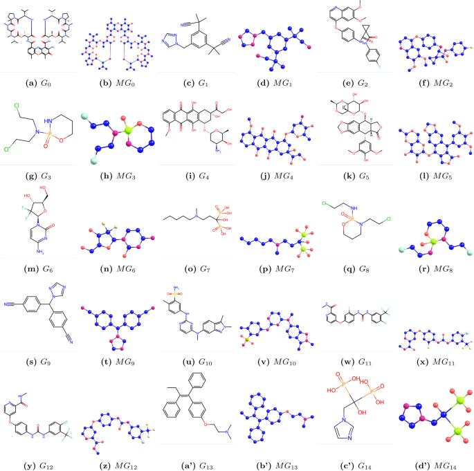
Graphs \(G_i\) and corresponding molecular graphs \(MG_i\) of bone drugs (\(i=0,1,\dots ,14\)).
Table 2 Physiochemical properties.
Theorem 1
Let \(G_0\) be the molecular graph of Actinomycin D, then the neighborhood M-polynomial is
\(NM(G_{0};x,y)=x^{2} y^{4} \left( 2 x^{5} y^{4} + 4 x^{4} y^{4} + 4 x^{4} y^{2} + 2 x^{3} y^{3} + 2 x^{3} y^{2} + 4 x^{2} y^{3} + 2 x^{2} y + x^{2} + 2 y\right) .\)
Proof
We consider the molecular graph of Actinomycin D and apply the neighborhood degree-based sum partition of its edges in the following form: \(|E_1{(2,5)}|\) =2, \(|E_2{(5,7)}|\) =2, \(|E_3{(4,7)}|\) =4, \(|E_4{(7,8)}|\) =2, \(|E_5{(6,8)}|\) =4, \(|E_6{(6,6)}|\) =4, \(|E_7{(5,6)}|\) =2, \(|E_8{(4,5)}|\) =2, \(|E_9{(4,4)}|\) =1,
Using the definition in equation (1), we substitute the partition of the edges into the equation and simplify. This gives:
$$\begin{aligned} NM(G_{0};x,y)= & \sum _{2\le 5}\lambda _{(2,5)}x^{2}y^{5} +\sum _{5\le 7}\lambda _{(5,7)}x^{5}y^{7} +\sum _{4\le 7}\lambda _{(4,7)}x^{4}y^{7} +\sum _{7\le 8}\lambda _{(7,8)}x^{7}y^{8} +\sum _{6\le 8}\lambda _{(6,8)}x^{6}y^{8}\\+ & \sum _{6\le 6}\lambda _{(6,6)}x^{6}y^{6} +\sum _{5\le 6}\lambda _{(5,6)}x^{5}y^{6} +\sum _{4\le 5}\lambda _{(4,5)}x^{4}y^{5} +\sum _{4\le 4}\lambda _{(4,4)}x^{4}y^{4}\\ M(G_{0};x,y)= & x^{2} y^{4} \left( 2 x^{5} y^{4} + 4 x^{4} y^{4} + 4 x^{4} y^{2} + 2 x^{3} y^{3} + 2 x^{3} y^{2} + 4 x^{2} y^{3} + 2 x^{2} y + x^{2} + 2 y\right) . \end{aligned}$$
\(\square\)
Theorem 2
Some topological indices for \(G_{0}=Actinomycin D\) are
\(M_1\) =264, \(M_2\) =17100, FN =1616, \(M_2^{nm}\) =18.9039, \(ND_3\) =9456, \(ND_5\) =49.85, NH =4.1949, NI =63.9522.
Proof
The NM-polynomial obtained in Theorem 1 and Table 1 is used to compute the indices, as:
$$\begin{aligned} Dx(NM)NM(G_{0};x,y)&= x^{2}y^{4} \left( 14 x^{5} y^{4} + 24 x^{4} y^{4} + 24 x^{4} y^{2} + 10 x^{3} y^{3} + 10 x^{3} y^{2} + 16 x^{2} y^{3} + 8 x^{2} y + 4 x^{2} + 4 y\right) ,\\ Dy(NM)NM(G_{0};x,y)&= x^{2} y^{4} \left( 16 x^{5} y^{4} + 32 x^{4} y^{4} + 24 x^{4} y^{2} + 14 x^{3} y^{3} + 12 x^{3} y^{2} + 28 x^{2} y^{3} + 10 x^{2} y + 4 x^{2} + 10 y\right) ,\\ Dx^2(NM)NM(G_{0};x,y)&= x^{2} y^{4} \left( 98 x^{5} y^{4} + 144 x^{4} y^{4} + 144 x^{4} y^{2} + 50 x^{3} y^{3} + 50 x^{3} y^{2} + 64 x^{2} y^{3} + 32 x^{2} y + 16 x^{2} + 8 y\right) ,\\ Dy^2(NM)NM(G_{0};x,y)&= x^{2} y^{4} \left( 128 x^{5} y^{4} + 256 x^{4} y^{4} + 144 x^{4} y^{2} + 98 x^{3} y^{3} + 72 x^{3} y^{2} + 196 x^{2} y^{3} + 50 x^{2} y + 16 x^{2} + 50 y\right) ,\\ Sx(NM)NM(G_{0};x,y)&= \frac{1}{420}[x^{2} y^{4} \left( 120 x^{5} y^{4} + 280 x^{4} y^{2} \left( y^{2} + 1\right) + 168 x^{3} y^{2} \left( y + 1\right) + 105 x^{2} \left( 4 y^{3} + 2 y + 1\right) + 420 y\right) ],\\ Sy(NM)NM(G_{0};x,y)&= \frac{1}{420}[x^{2} y^{4} \left( 105 x^{4} y^{4} \left( x + 2\right) + 140 x^{3} y^{2} \left( 2 x + 1\right) + 120 x^{2} y^{3} \left( x + 2\right) + 105 x^{2} + 168 y \left( x^{2} + 1\right) \right) ],\\ J(NM)NM(G_{0};x,y)&= x^{7} \left( 2 x^{8} + 4 x^{7} + 6 x^{5} + 6 x^{4} + 2 x^{2} + x + 2\right) . \end{aligned}$$
\(\square\)
The NM-polynomials for other drug structures from \(G_{1}\) to \(G_{14}\) can be obtained similarly to the proof of Theorem 1 and are shown in Table 3.
\(G_{1}\)= Anastrozole; \(G_{2}\)= Cabozantinib; \(G_{3}\)= Cyclophosphamide; \(G_{4}\)= Doxorubicin; \(G_{5}\)= Etoposide; \(G_{6}\)= Gemcitabine; \(G_{7}\)= Ibandronate; \(G_{8}\)= Ifosfamide; \(G_{9}\)= Letrozole; \(G_{10}\)= Pazopanib; \(G_{11}\)= Regorafenib; \(G_{12}\)= Sorafenib; \(G_{13}\)= Tamoxifen; \(G_{14}\)= Zoledronic acid; we have:
$$\begin{aligned} NM(G_1;x,y)&= x^{2} y^{4}(2 x^{5} y^{4} + 4 x^{4} y^{4} + 4 x^{4} y^{2} + 2 x^{3} y^{3} + 2 x^{3} y^{2} + 4 x^{2} y^{3} + 2 x^{2} y + x^{2} + 2 y),\\ NM(G_2;x,y)&= x^{2} y^{4}(2 x^{5} y^{6} + 2 x^{5} y^{4} + x^{5} y^{3} + 2 x^{4} y^{6} + x^{4} y^{4} + 6 x^{4} y^{3} + 4 x^{4} y^{2} + 2 x^{3} y^{3} + 6 x^{3} y^{2} + 6 x^{3} y \\&+ 2 x^{2} y^{3} + 2 x^{2} y + 2 x y^{3} + x y + 2),\\ NM(G_3;x,y)&= x^{2} y^{3} (x^{6} y^{5} + 2 x^{4} y^{5} + 2 x^{3} y^{5} + x^{2} y^{5} + 2 x^{2} y^{3} + 2 x^{2} y + 2 x y^{2} + 2),\\ NM(G_4;x,y)&= x^{2} y^{4} (x^{7} y^{5} + 2 x^{6} y^{5} + 8 x^{5} y^{5} + 6 x^{5} y^{4} + x^{5} y^{3} + 3 x^{4} y^{3} + 5 x^{4} y^{2} + x^{3} y^{4} + x^{3} y^{3} + x^{2} y^{4} + 2 x^{2} y^{3} + 2 x^{2} y\\&+ 6 x y^{3} + 2 x y^{2} + 2),\\ NM(G_5;x,y)&= x^{2} y^{4} (x^{7} y^{5} + 2 x^{6} y^{5} + 3 x^{6} y^{4} + x^{5} y^{5} + 2 x^{5} y^{4} + 5 x^{5} y^{3} + x^{4} y^{5} + 4 x^{4} y^{4} + 9 x^{4} y^{3} + x^{3} y^{4} + 3 x^{3} y^{3}\\&+ 2 x^{3} y^{2} + 3 x^{3} y + 2 x^{2} y^{3} + 2 x^{2} y + 3 x y^{3} + x y^{2} + x y + 2),\\ NM(G_6;x,y)&= x^{2} y^{4} (2 x^{6} y^{5} + x^{6} y^{4} + x^{5} y^{4} + x^{4} y^{5} + x^{4} y^{4} + x^{4} y^{3} + x^{4} y^{2} + x^{3} y^{4} + x^{3} y^{2} + 2 x^{3} y + 2 x^{2} y^{4} + x^{2} y^{3}\\&+ x y^{4} + x y^{2} + x y + 1),\\ NM(G_7;x,y)&= x^{2} y^{3} (2 x^{5} y^{8} + x^{4} y^{8} + x^{3} y^{3} + 2 x^{3} y^{2} + x^{2} y^{8} + 6 x^{2} y^{4} + x^{2} y^{2} + x^{2} y + x y^{2} + x y + 1),\\ NM(G_8;x,y)&= x^{2} y^{3} (x^{6} y^{5} + 2 x^{4} y^{5} + 2 x^{3} y^{5} + x^{2} y^{5} + 2 x^{2} y^{3} + x^{2} y^{2} + x^{2} y + x y^{2} + x y + 2),\\ NM(G_9;x,y)&= x^{2} y^{4} (3 x^{5} y^{5} + 6 x^{3} y^{3} + 4 x^{3} y^{2} + 4 x^{3} y + 2 x^{2} y^{2} + 2 x^{2} y + x^{2} + 2),\\ NM(G_{10};x,y)&= x^{3} y^{5} (2 x^{4} y^{3} + 2 x^{4} y^{2} + 3 x^{3} y^{4} + 5 x^{3} y^{2} + 5 x^{3} y + x^{2} y^{3} + 2 x^{2} y^{2} + 3 x^{2} y + 2 x^{2} + 3 x y + 2 x + 2 y^{2} + 2 y),\\ NM(G_{11};x,y)&= x^{2} y^{4}(3 x^{4} y^{5} + 4 x^{4} y^{3} + 7 x^{4} y^{2} + 2 x^{3} y^{3} + 6 x^{3} y^{2} + 2 x^{3} y + 4 x^{2} y^{2} + 2 x^{2} y + 3 x y^{2} + x y + 1),\\ NM(G_{12};x,y)&= x^{2} y^{4} (3 x^{4} y^{5} + 2 x^{4} y^{3} + 6 x^{4} y^{2} + x^{3} y^{3} + 9 x^{3} y^{2} + 3 x^{3} y + 4 x^{2} y^{2} + 2 x^{2} y + 2 x y^{2} + x y + 1),\\ NM(G_{13};x,y)&= x^{2} y^{4} (x^{6} y^{5} + 2 x^{5} y^{5} + x^{5} y^{4} + 6 x^{3} y^{3} + 3 x^{3} y^{2} + 2 x^{3} y + x^{2} y^{4} + 7 x^{2} y + 4 x^{2} + 2 x + 1),\\ NM(G_{14};x,y)&=x^{4} y^{4} (3 x^{3} y^{7} + x^{2} y^{3} + 2 x y^{2} + y^{7} + 6 y^{3} + 2 y + 1). \end{aligned}$$
Table 3 Different toplogical indices.Table 4 Statistical parameters and regression models for \(M_1(G)\).Fig. 2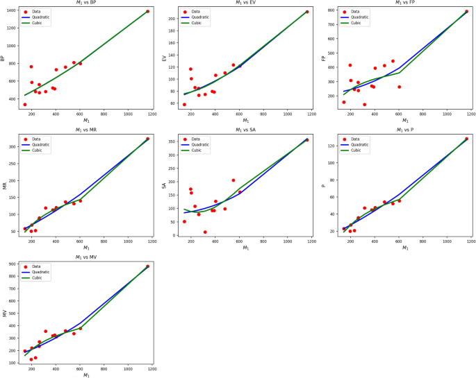
Scatter plots of actual data points (red) and regression model fits (Quadratic in blue, cubic in green) for various drug response parameters versus \({M_1(G)}\).
Table 4 also evaluates the association between M1(G) and drug-response metrics using quadratic and cubic regression models. Quadratic models systematically perform better than their cubic equivalents, as indicated by higher R values (0.837 0.974) and significantly greater \(R^2\) values. Cubic BP, EV, and FP models are weak in comparison, with \(R^2\) values as low as 0.184 for EV, implying limited explanatory capacity of this predictor in the cubic models. The standard error is also lower in almost all quadratic models, reflecting improved predictive accuracy.
F-statistics also add weight to the quadratic models’ reliability, with particularly high values observed in the cases of MR, P, and MV, implying strong general significance. All p-values of the quadratic models are well below 0.001, supporting their statistical validity, while some p-values of the cubic models reach or surpass 0.05, undermining their credibility. Figure 2 corroborates the statistical results through the visualization of regression fits over actual data points. The blue curves of the quadratics closely track the red data points, particularly in sequences such as MR, P, and MV, where the alignment is nearly perfect. The green curves of the cubics, conversely, tend to diverge unnecessarily, yielding poor fits in regions with low data density. This visual confirmation reinforces the numerical results, establishing that drug response as a function of \(M_1(G)\) is better represented by quadratic models than by cubic ones due to improved fit and reduced error rates.
Table 5 Statistical parameters and regression models for \(M_2(G)\).Fig. 3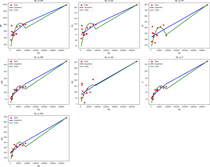
Scatter plots of actual data points (red) and regression model fits (Quadratic in blue, cubic in green) for various drug response parameters versus \({M_2(G)}\).
Table 5 also evaluates the association between \(M_2(G)\) and drug response metrics through quadratic and cubic regression models. Quadratic models systematically perform better than their cubic counterparts, as indicated by superior R values (0.837 to 0.974) and significantly higher \(R^2\) values. Cubic BP, EV, and FP models are weak in comparison, with\(R^2\) as low as 0.184 being achieved by EV, implying weak explanatory capacity of this predictor in the cubic models. The standard error is also lower in almost all of the quadratic models, reflecting improved predictive accuracy. F-statistics further support the reliability of the quadratic models, with particularly high values observed in the cases of MR, P, and MV, indicating strong general significance. All p-values of the quadratic models are well below 0.001, affirming their statistical validity, while several cubic model p-values meet or exceed 0.05, diminishing their credibility. Figure 3 confirms the statistical results through visual regression fits on actual data points. The blue curves of the quadratics closely follow the red data points, especially in sequences like MR, P, and MV, where alignment is nearly flawless. In contrast, the green cubic curves tend to deviate unnecessarily, producing poor fits in data-sparse areas. The visual confirmation supports the numerical results, thereby establishing that drug response as a function of \(M_2(G)\) is better represented by quadratics than cubics, through improved fit and reduced error rate.
Table 6 Statistical parameters and regression models for FN(G).Fig. 4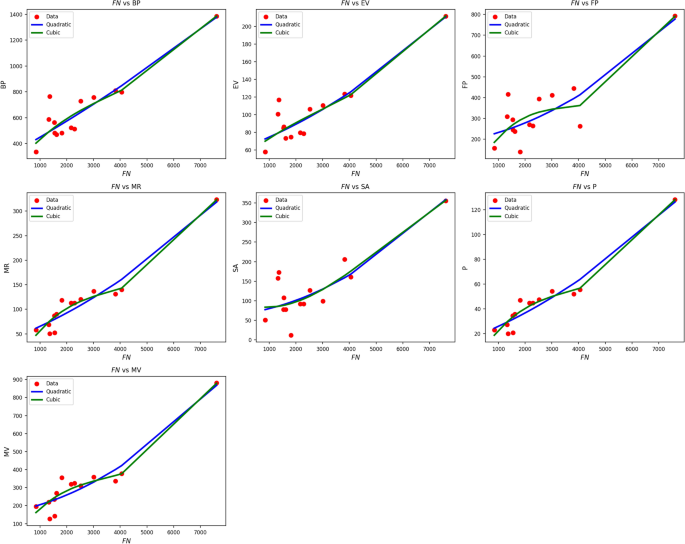
Scatter plots of actual data points (red) and regression model fits (quadratic in blue, cubic in green) for various drug response parameters versus FN(G).
Table 6 explores the impact of FN(G) on drug response criteria using both quadratic and cubic regression models. Quadratic models are highly predictive, with R values between 0.854 and 0.967, and \(R^2\) values well over 0.72. Notably, the MR and P parameters exhibit \(R^2\) values above 0.93, reflecting excellent explanatory capability. Although the cubic models produce slight improvements in R and \(R^2\) for some variables such as MR (increasing from 0.934 to 0.955) and FP (from 0.729 to 0.758) these gains are offset by increased standard deviations, which signify reduced precision. All models yield statistically significant results, with p-values well below 0.005. F-measures are high, especially for MR and P, highlighting the robustness of the models. Overall, quadratic models offer a good trade-off between high correlation, low error, and simplicity, making them the preferred method when studying FN(G). Figure 4 provides a visual comparison of actual data points versus model projections for FN(G). The red data points are closely matched by the blue quadratic curve in most cases, particularly for MR, P, and MV, thereby replicating the superior statistical outcome. The cubic curves (green) offer minor improvements in curvature but tend to overfit in sparse data regions. Overall, the visual correspondence and consistent statistical results confirm that quadratic modeling is highly successful and superior to cubic modeling when analyzing drug response versus FN(G).
Table 7 Statistical parameters and regression models for \(ND_3(G)\).Fig. 5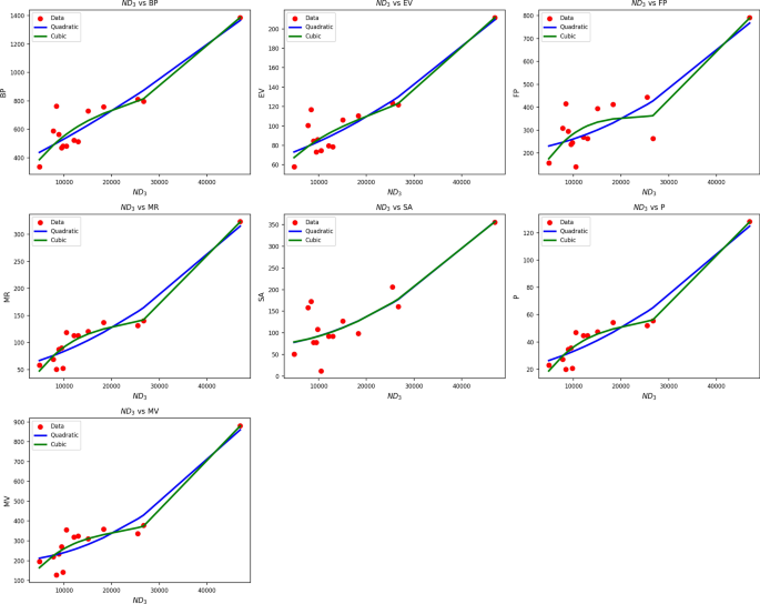
Scatter plots of actual data points (red) and regression model fits (Quadratic in blue, cubic in green) for various drug response parameters versus \({ND_3(G)}\).
Table 7 shows regression statistics relating drug response parameters to \(ND_3(G)\) using both quadratic and cubic modeling. Both models show excellent fits, with high R values (quadratic: 0.847 to 0.952; cubic: up to 0.971) and significant \(R^2\) values, indicating high levels of correlation. Notably, MR and P have \(R^2\) values of 0.907 to 0.943, implying that \(ND_3(G)\) can be used as a reliable predictor for these endpoints. While in some cases cubic models can improve \(R^2\), e.g., MR (0.943 vs. 0.907) they tend to be associated with greater standard error. For example, SE increases from 0.002 to 0.006 for MR, which can reduce predictive consistency. p-values are highly significant across all variables \((p , verifying the quality of both models. Nevertheless, considering the trade-off between model complexity and predictive performance, the quadratic models have the advantage of being more stable and interpretable, with fewer parameters and consistently strong performance across drug response types. Figure 5 schematically confirms the quantitative findings. The blue quadratic curves closely follow the red data points in all response parameters, especially for MR, P, and MV, with high fidelity to observation. The green cubic curves, though slightly more adaptable, diverge in less densely covered regions, where overfitting becomes more likely. This corroborates the conclusion that quadratic models provide accurate, transferable predictions by \(ND_3(G)\) while remaining simple and precise in describing the drug response profile.
Table 8 Statistical parameters and regression models for \(ND_5(G)\).Fig. 6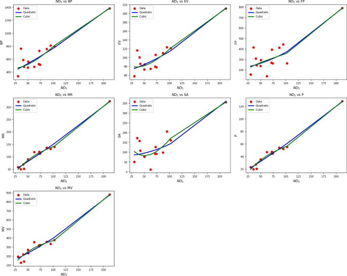
Scatter plots of actual data points (red) and regression model fits (quadratic in blue, cubic in green) for various drug response parameters versus NH(G).
Table 8 assesses the association between \(ND_5(G)\) and drug response parameters through quadratic and cubic regression analysis. Both models generate high R and \(R^2\) values, indicating strong associations across all parameters. Of particular note are the very high \(R^2\) values of MR and P in both models 0.976 in the quadratic and 0.983 in the cubic implying very high predictive capability. Nevertheless, cubic models tend to have greater standard errors, which may imply overfitting. The SE, for example, increases significantly from 2.785 (quadratic) to 15.530 (cubic) in the case of BP, and the same pattern is observed in other parameters such as EV and FP. Although the cubic models increase \(R^2\) slightly, the accompanying rise in SE tends to reduce their usefulness in practice. All models retain high F-values and statistically highly significant p-values \((p , endorsing their validity. However, since the improvement in explanatory ability is modest and the increase in error is greater, the quadratic models present a superior trade-off between precision and simplicity in most drug response prediction contexts involving \(ND_5(G)\). Figure 6 provides supporting evidence with clear visualizations. The quadratic model (blue line) closely follows the pattern of actual data points (red), especially for MR, P, and MV, where the fit is nearly exact. The cubic model (green) may offer more flexibility but oscillates excessively in low-density regions, indicating instability. Overall, both visual and statistical evidence consistently indicate the quadratic model as the more useful and stable choice for modeling drug responses.
Table 9 Statistical parameters and regression models for NH(G).Fig. 7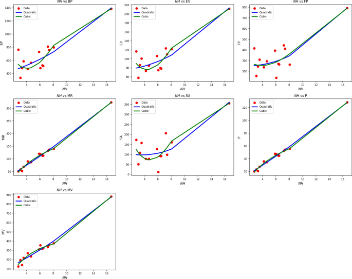
Scatter plots of actual data points (red) and regression model fits (quadratic in blue, cubic in green) for various drug response parameters versus NH(G).
Table 9 shows regression results of NH(G) on drug response measures with quadratic and cubic models. Both model forms produce statistically significant results, with p-values less than 0.005 and high F-statistics across the board. Parameters like MR, P, and MV have very high R values of up to 0.995 and 0.997, indicating high correlation. Cubic models improve \(R^2\) values slightly, such as when MR increases to 0.993 from 0.990, but this tends to come at the expense of greater standard error. SE, for instance, increases dramatically from 41.999 in the quadratic form to 291.420 in the cubic form, meaning less reliable estimations. Overall, while cubic forms can better fit nonlinear curves, they add more variability and complexity without providing proportional increases in fit. Therefore, quadratic models generate more stable, interpretable, and more efficient solutions for assessing the impact of drug responses by NH(G). Figure 7 reinforces these results. Quadratic fits (blue lines) closely follow actual data (red squares) for most parameters, e.g., MR, MV, and P. Cubic models (green lines) diverge or over-curve in some areas, particularly where data are sparse or less variable. These over-swings indicate overfitting in some data sets, even with slight \(R^2\) improvements. Both visually and statistically, the quadratic model offers a smoother, more regular portrayal of the drug response behavior associated with NH(G) and, as such, represents the better option when performing predictive modeling in this genomic context.
Table 10 Statistical parameters and regression models for NI(G).Fig. 8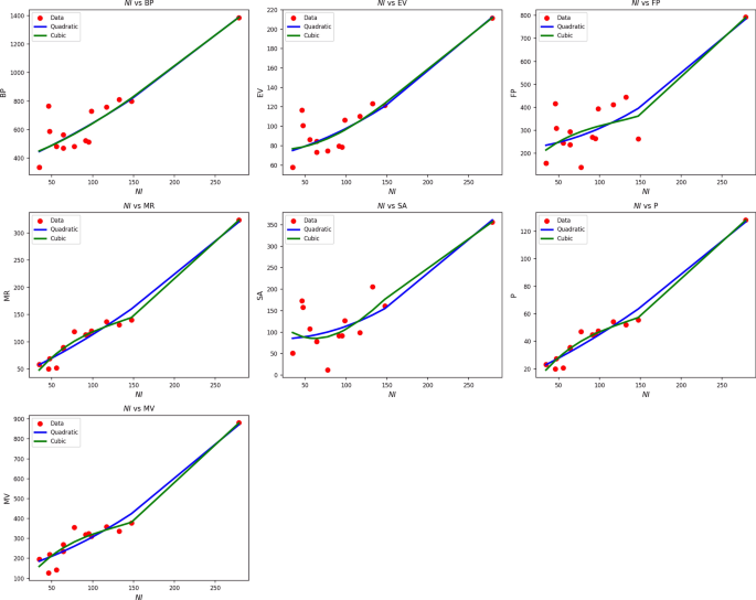
Scatter plots of actual data points (red) and regression model fits (quadratic in blue, cubic in green) for various drug response parameters versus NI(G).
Table 10 assesses the impact of NI(G) on different drug response parameters through both the quadratic and cubic regression models. The findings reveal excellent fits of the models to all responses, with R values well over 0.90 and \(R^2\) well over 0.82 in most of the quadratic models. Notably, MR, P, and MV show very good predictability with quadratic \(R^2\) values of 0.963, 0.963, and 0.934, respectively. Although the cubic models improve \(R^2\) slightly, e.g., to 0.975 in the case of MR, the concomitant increase in standard error lowers their predictive clarity. The SE, for example, rises from 1.861 to 8.461 when moving from quadratic to cubic, respectively. Although both models yield highly significant p-values \((p , the SE levels are consistently lower in the quadratic models, implying greater predictive reliability with reduced risk of overfitting. F-values are particularly large for MR, P, and MV, confirming the robustness of both models. Nevertheless, the superior trade-off between simplicity, accuracy, and stability makes the quadratic form the better choice to represent the impact of NI(G). Figure 8 reinforces these findings visually. Quadratic curves (blue) closely follow the red actual data points, particularly in the cases of MR, P, and MV, where the fits are tight and stable. Cubic fits (green), while more flexible, tend to veer off or oscillate more widely, especially in regions of sparse data. Both visual and statistical analyses, therefore, verify the quadratic model as the most reliable paradigm for representing drug responses as a function of NI(G), offering strong, stable, and meaningful results.