
Device architecture and cluster state generation protocol
To generate ladder-like cluster states, we use two transmon qubits whose lowest three levels we label \(\vert g\rangle\), \(\vert e\rangle\) and \(\vert \, f\rangle\), tunably coupled to each other33. We refer to these as ‘source qubits’, S1 and S2. In addition, each source qubit is tunably coupled to a waveguide, allowing for controlled emission of photons Pi, see Fig. 1a. To generate multipartite entangled states, S1 and S2 are entangled and subsequently emit itinerant photonic qubits Pi (red and blue photon envelopes) sequentially. The procedure is repeated many times to generate 2 × n ladder-like cluster states. We implement this scheme with a device consisting of four superconducting transmon qubits as shown in Fig. 1b. The source qubits S1 (red) and S2 (blue) are transmon qubits with fixed \(\vert g\rangle \leftrightarrow \vert e\rangle\) transition frequencies of 5.589 GHz (S1, T1 = 27 μs, \({T}_{2}^{*}=22\,\mu {{{{\rm{s}}}}}\)) and 5.619 GHz (S2, T1 = 22 μs, \({T}_{2}^{*}=23\,\mu {{{{\rm{s}}}}}\)). We realize the tunable coupling to a common waveguide for each source qubit via a frequency-tunable emitter qubit (brown, E1 at 5.754 GHz and E2 at 5.354 GHz) and a tunable coupler (orange, C1 and C2). The emitter qubits are strongly coupled to the common waveguide, such that any excitation of the emitter qubits rapidly decays into the waveguide as an itinerant photonic qubit with characteristic decay times of T1 = 2/κ = 54 ns (E1) and 42 ns (E2). The coupling between the source qubits is also realized by a tunable coupler, CSS. The tunable couplers consist of two parallel coplanar waveguides (CPWs) coupling two neighboring qubits19,26,34. One CPW has a superconducting quantum interference device (SQUID) placed in the middle of the center conductor allowing flux-tuning of the CPW’s inductance and thus its effective electrical length. Choosing a particular bias, we can utilize destructive interference between the fields propagating along each path to cancel the interaction between the two qubits19,26,34. By modulating the flux threading the SQUID loop using a flux line, we parametrically drive the sideband transitions illustrated in Fig. 1c–e, enabling two-qubit gates19,34,35,36.
Figure 1f shows the quantum circuit used to generate a 2 × n ladder-like cluster state18. The protocol begins with a Hadamard gate on both S1 and S2 followed by a CZ gate between these two qubits. To implement the CZ gate, we parametrically drive a 2π rotation on the \(\vert ee\rangle \leftrightarrow \vert \, fg\rangle\) transition35, as illustrated in Fig. 1c. This imparts a conditional relative geometric phase between the two qubits35,37. The phase accumulated depends on the detuning of the \(\vert ee\rangle \leftrightarrow \vert \, fg\rangle\) pulse38—a resonant pulse results in a phase shift of π, thus enacting a CZ gate. The CZ gate is followed by controlled emission of a photonic qubit from S1 and S2 via CNOT gates. We perform two-qubit gates between a source qubit S1 or S2 and a photonic qubit Pi by using the emitter qubits, whose lowest two levels we label \(\vert 0\rangle\) and \(\vert 1\rangle\). The CNOT gate, shown in Fig. 1d, is realized by first performing a πef rotation on the source qubit and then parametrically driving the \(\vert \, f0\rangle \leftrightarrow \vert e1\rangle\) transition19,36. If excited, the emitter subsequently decays into the waveguide, emitting an itinerant microwave photon25,27. A photon is only emitted if the source qubit is initially in \(\vert e\rangle\), realizing a CNOT gate between the source and the emitted photonic qubit. For the emission of the first n − 1 pairs of photons a gate sequence consisting of Hadamard-CZ-CNOT is repeated n − 1 times. In the last emission step, emission of the photonic qubits is done via a SWAP gate from S1 to E1 and from S2 to E2 instead of a CNOT gate. We perform such a SWAP gate by transferring the excitation into the emitter qubit by parametrically driving the \(\vert e0\rangle \leftrightarrow \vert g1\rangle\) transition19,36, as shown in Fig. 1e. These final SWAP gates disentangle S1 and S2 from the generated entangled photonic state. With this protocol, in every emission step a pair of photonic qubits is generated simultaneously, i.e., their temporal modes start at the same time, but at different frequencies, resulting in a 2 × n ladder-like cluster state. Note that even though the photonic qubits’ envelopes start simultaneously, the shape and duration of the envelope is different, due to the different coupling rates for S1 and S2.
To reduce cross-talk between the source qubits, which are detuned by less than 30 MHz (due to a frequency targeting error while fabricating the chip), we choose to perform single qubit gates acting on either S1 or S2 in 128 ns, slower than state-of-the-art39,40, thereby decreasing the spectral overlap between the drive pulses. For the two-qubit gates, which are unaffected by the small detuning between the source qubits, we optimize gate times resulting in a 173 ns CZ gate. We perform the CNOT gates in 110 ns (S1) and 106 ns (S2), and the SWAP gates in 186 ns (S1) and 240 ns (S2). To ensure the emitter qubits fully decay to their ground state after a SWAP or CNOT gate, we choose a 650 ns delay between successive emission of photon pairs in our protocol. All relevant device parameters are summarized in Supplementary Note 1, Supplementary Table S1. Further details of the detection scheme and experimental setup are given in Supplementary Note 1.
State characterization
When generating an entangled photonic state, the emitted photons Pi propagate into the common waveguide and are routed off chip into a coaxial output line. The microwave photons are then amplified and their quadratures are measured at room temperature41,42. Note that the amplification is necessary due to the low energy of microwave photons (ℏω/kB ~ 100 mK), but adds noise, limiting the quantum efficiency η to around 0.25 in our state-of-the-art setup. Alternatively, one could noiselessly detect microwave photons using custom-made microwave photon detectors43,44,45. Here, we choose to characterize the radiation using amplification for simplicity. We characterize the emitted photonic modes Pi by recording their respective quadratures Ii and Qi42. From Ii and Qi, we then calculate statistical moments \(\langle {\hat{a}}^{{{{\dagger}}} s}{\hat{a}}^{t}\rangle\)27 of the emitted photonic modes Pi. As we are interested in the statistical moments of the photonic modes when emitted from the superconducting device, we calibrate out the noise added by the amplification chain27,41 as detailed in Supplementary Note 3, which makes use of the linearity of the amplification chain. Noise added during amplification therefore does ideally not affect the fidelity of the reconstructed density matrix, but rather decreases the detection efficiency η. As we find that the second order correlation \(\langle {\hat{a}}^{{{{\dagger}}} 2}{\hat{a}}^{2}\rangle\) is close to zero, confirming the linearity of the detection chain (see Supplementary Note 3 for details), we truncate the Hilbert space to s, t ∈ {0, 1}, i.e., the single photon Hilbert space. To then reconstruct the density matrix of up to 4-qubit states from the integrated quadratures, we calculate joint moments \(\langle {\hat{a}}_{1}^{{{{\dagger}}} s}{\hat{a}}_{1}^{t}{\hat{a}}_{2}^{{{{\dagger}}} u}{\hat{a}}_{2}^{v}{\hat{a}}_{3}^{{{{\dagger}}} w}{\hat{a}}_{3}^{x}{\hat{a}}_{4}^{{{{\dagger}}} y}{\hat{a}}_{4}^{z}\rangle\), where s, t, . . . , z ∈ {0, 1}, of all constituent photonic qubits Pi and perform maximum likelihood estimation on the extracted moments to obtain the most likely physical density matrix5,42, see Supplementary Note 4 for details.
As the number of required measurement runs to achieve a given signal-to-noise ratio k ∝ 1/ηO, where η is the quantum efficiency of the detection chain, scales exponentially with the order O of the moment41, measuring joint moments of more than four photonic qubits becomes challenging. Thus, for states consisting of more than four photonic qubits, we use a two-step reconstruction process. Qubits in the generated states have at most 3 nearest neighbors. We reconstruct the density matrices of all four-qubit subsets of the generated state consisting of each qubit and its nearest neighbors. From these we efficiently reconstruct a matrix product operator representing the full density matrix, as described in ref. 28, making use of the fact that the cluster state is the unique ground state of a gapped nearest-neighbor Hamiltonian46. The algorithm iteratively finds the most likely state consistent with the reduced density matrices, see Supplementary Note 4 for details. For imperfect cluster states, the efficient tomography method introduces errors, as the reduced density matrices do not uniquely specify the global state. Therefore, the density matrices reconstructed with the efficient tomography method are only approximations to the actual density matrices. We investigate the fidelity between the reconstructed and the actual state further in Supplementary Note 4 using master equation simulations. We find that, for simulated imperfect cluster states, the fidelity between the reconstructed and the actual state drops with the size of the cluster state, indicating larger reconstruction errors in the larger reconstructed cluster states.
To illustrate the generation of the cluster states step by step, and to demonstrate the flexibility of the device in generating different states, we generate three states each consisting of six photons, each using a different number of entangling gates. The quantum circuits used to generate these three states are shown in Fig. 2a, c, e. In Fig. 2b, d, f, we show the reconstructed density matrices of these states, whose entanglement structure is illustrated in the insets. In (a, b), we perform only a single CZ entangling gate in the first emission step, followed by SWAP gates. In the other emission steps, we only apply Hadamard and SWAP gates, thus not creating entanglement. In (c, d), we add additional CHPASE and CNOT gates to create a four-qubit cluster state in a six-qubit subspace. Finally, in (e, f), we perform the full sequence of gates to generate a six-qubit cluster state. In each step we see that the addition of more entangling gates introduces additional structure to the density matrix, resulting in the intricate pattern of stripes in Fig. 2f that corresponds to a six-qubit cluster state. We choose to display the real part of the density matrix in Fig. 2b, d, f as the imaginary part (see Supplementary Note 4), which for an ideal cluster state would be zero, contains mostly noise due to dephasing and gate qubit errors and is on average about five times smaller than the real part.
Fig. 2: Step by step build-up of a six-qubit cluster state.
We prepare six photonic qubits in three separate experiments, starting with a gate sequence containing only one entangling CZ gate (a), four entangling gates (c), and finally the full sequence to generate a six-qubit cluster state (e). The resulting reconstructed density matrices are shown in (b, d, f), below the corresponding gate sequences. For each density matrix an illustration of the entanglement structure is also depicted in the upper-right corner.
We performed the 2 × n-qubit cluster state generation protocol outlined above for n ∈ {2, 3, 4, …, 10}, resulting in cluster states of up to 20 photonic qubits. We find that the reconstructed N-photon cluster state density matrices ρExp have fidelities \(F={{{{\rm{Tr}}}}}{(\sqrt{{\rho }_{{{{{\rm{Exp}}}}}}{\rho }_{{{{{\rm{Ideal}}}}}}})}^{2}\) of 0.84 (four qubit), 0.77 (six qubit), 0.59 (eight qubit) and 0.12 (20 qubit) to the corresponding ideal cluster state ρIdeal (see Supplementary Note 4 for more details). For the four, six and eight qubit states, the fidelity therefore exceeds the threshold for genuine multipartite entanglement of 50%, i.e., the generated state cannot be written as a convex sum of bi-separable states47.
The density matrix of the 20 qubit cluster state, containing a total of 240 ≈ 1 × 10¹² entries, is too large to display and impractical to construct as a density matrix in full, so we instead reconstruct the state entirely in the matrix product operator representation and only show the upper-left part and far off-diagonal part of the density matrix, see Fig. 3a, b for the phase and Supplementary Note 4 for the magnitude. We observe that for all cluster state density matrices for N = 2, 4, . . . , 20, including those not shown, elements closer to the \(\vert 00…\rangle\) state are larger in magnitude compared to the ideal state while far off-diagonal elements are smaller in magnitude than the ideal state. This is due to source qubit decay and dephasing occurring during the execution of the protocol (see Supplementary Note 4). As this dephasing causes the diagonal elements of \({{{{\rm{Re}}}}}(\rho )\) to be much larger than the off-diagonal elements, we instead plot the phase in Fig. 3a, b, which emphasizes the patterns in the phase stemming from entanglement more clearly. The patterns in Fig. 3a are not strongly affected by dephasing, as they reflect local correlations, for which the effect of dephasing is small. For the far off-diagonal elements in Fig. 3b, the patterns are also locally correct, however when comparing to the ideal state, we notice errors in relative phase between distant qubits, likely a consequence of control errors.
Fig. 3: Sections of the density matrix of a 20 photonic qubit state.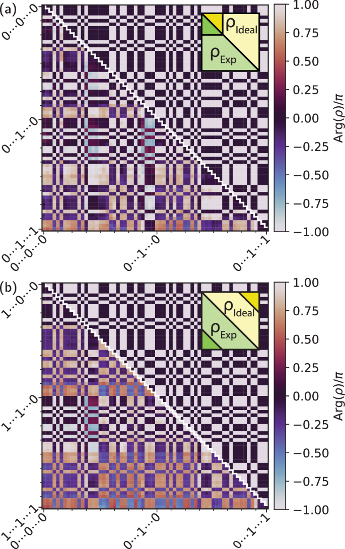
Phase of the experimental ρExp (below diagonal) and the ideal ρIdeal (above diagonal) density matrix of the 20 qubit cluster state, showing only (a) the upper-left part and b far off-diagonal part of the full density matrix. Darker colored triangles in the insets indicate the sections of the density matrix displayed.
To further characterize the generated multi-qubit states, we estimate up to which number of qubits measurable entanglement persists across the multi-qubit state. Fidelity primarily measures how close a state is to a target state, and for states whose fidelity is less than 50% to the target state we cannot make a statement about entanglement anymore. For example, a state can be maximally entangled, but differ from the target state by single-qubit gates, rendering the fidelity to be close to 0. However, there are several metrics aimed at measuring multipartite entanglement2, and we choose to use localizable entanglement, as it is commonly used14,19. The localizable entanglement metric is also closely related to important applications like measurement-based quantum computing or error-corrected quantum communication, as obtaining the localizable entanglement metric requires measuring all but two qubits in certain bases. We thus expect that the localizable entanglement metric is indicative of the performance of generated cluster states in the context of measurement-based quantum computing or error-corrected quantum communication.
We calculate the localizable entanglement between the first P1 and last PN photonic qubit48,49. To do so, we project all other qubits either in the X or the Z basis and then evaluate the negativity between P1 and PN. For a cluster state a Z projection removes the node and its bonds, while an X projection preserves the entanglement bonds49. We apply these projections to the reconstructed state in post-processing. Using X projections, we construct a path of length n = N/2, the shortest possible distance, between P1 and PN, while applying Z projections on all nodes outside the path; see Supplementary Note 8 for details. Figure 4a illustrates an example path for N = 10. As each projection has a probabilistic outcome, for an N-qubit state, there are 2N−2 possible outcomes for each path. For states larger than N = 12 it becomes impractical to compute all such outcomes. We therefore average the obtained negativity over 1024 randomly sampled projection outcomes and obtain the localizable entanglement for each path, then average over all paths with length n = N/2. A nonzero localizable entanglement value indicates that there is measurable entanglement between P1 and PN.
Fig. 4: Quantifying entanglement of the generated states.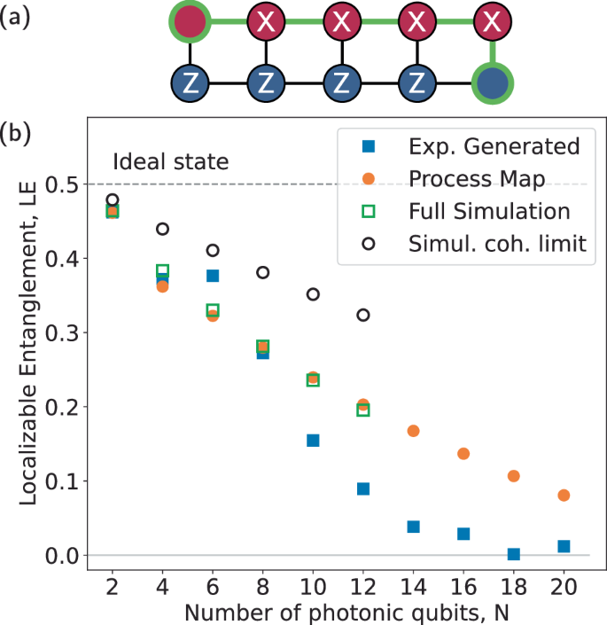
a Schematic illustrating the chosen localizable entanglement metric for a 10 photonic qubit state. Qubits are projected into either the X or the Z bases, as indicated, then localizable entanglement is calculated for the two corner qubits (green edges). b Localizable entanglement as a function of number of generated photonic qubits N = 2 × n, as measured by matrix product operator tomography of the experimentally generated states (exp. generated, blue, solid squares), as estimated from process maps (orange, solid circles), and as obtained by master equation simulations taking into account all errors (green, empty squares) and only decoherence (simul. coh. limit (simulated coherence limit), black, open circles), and the localizable entanglement of the ideal state (gray, dashed line). Shown is the mean over all possible paths of length n.
We calculate the localizable entanglement for experimentally generated and reconstructed states. However, as errors introduced by the efficient tomography method increase for larger, imperfect cluster states (see Supplementary Note 4 for details), we employ an additional complementary method to verify the results. We measure process maps of the two repeated processes (H followed by CZ and CNOT or H followed by CZ and SWAP) using process tomography. Assuming that the emission process applied does not change when photonic qubits are emitted sequentially, we repeatedly apply the extracted process maps to the initial ground state density matrix \(\vert gg\rangle \langle gg\vert\) of the source qubits to calculate the expected density matrix of the generated cluster states11,19, see Supplementary Note 6 for further details. Inferring the density matrix from the reconstructed process map assumes a repeatable process with time-independent error. In our experiment, this assumption appears to be well justified because both the microwave frequency control pulses and the system parameters are found to be stable over the microsecond timescales of individual sequences. From these density matrices we can also extract the localizable entanglement for comparison. Finally, we perform two types of master equation simulation of the state generation sequence, one taking into account only decay and dephasing errors, estimated from measured source qubit \({T}_{1},{T}_{2}^{*}\) values, and one taking into account all errors (i.e., including coherent gate errors), see Supplementary Note 7 for further details. From these simulations, we extract the localizable entanglement from the resulting simulated density matrices. The localizable entanglement values calculated from all above methods for states up to 20 photons in size are shown in Fig. 4. We see that the localizable entanglement gets smaller with increasing state size for all data and analyses. This is expected as larger system sizes involve longer gate sequences and therefore more decoherence and gate errors. The simulations including only decay and dephasing have larger localizable entanglement than those taking into account all errors, indicating that coherent gate errors make a significant contribution to the overall error in state generation. The localizable entanglement extracted from process maps agrees well with the simulation including all errors, while the experimentally generated and reconstructed density matrices for N > 8 yield localizable entanglement values significantly below that of the process maps and simulations. This is most likely due to errors introduced by the efficient tomography method. To verify this, we apply the efficient tomography method to density matrices obtained from master equation simulations and observe a reduction in the extracted localizable entanglement and fidelity of the reconstructed density matrices compared to the simulated density matrices, which do not require reconstruction, see Supplementary Note 4 for details. The efficient tomography method thus, at least for the simulated states, results in a conservative estimate of the localizable entanglement. In addition, both the results from process tomography as well as simulations indicate a larger localizable entanglement. Using the most conservative localizable entanglement estimate obtained with the three reconstruction methods, we see that the localizable entanglement is nonzero for states comprising up to 16 qubits, and drops to near-zero for the measured 18- and 20-qubit states. On the other hand, the process tomography does not suffer from the limitations of the efficient tomography methods for reconstructing large and imperfect cluster state, and predicts that entanglement should persist for even larger states.
From the analysis of process maps and master equation simulations, we conclude that the ultimate size of the states we can generate is limited both by the fidelity of our single and two-qubit gates and from decoherence during the pulse sequence. Qubit drive-line crosstalk is likely primarily responsible for the single qubit gate error and crosstalk cancellation should alleviate this. Further optimization of the coupler design and qubit frequencies and fine-tuning of the gate parameters may be feasible to increase two-qubit gate (in particular, the CZ gate) fidelities, which we, using simulations, estimate to currently be around 97%, towards the state-of-the-art performance for similar tunable coupler designs50. Extending qubit coherence times from 22 μs (S1) and 23 μs (S2) towards the state of the art, which is more than an order of magnitude longer51, will reduce the decoherence-related error that we observe in the largest states generated. This will permit the utilization of significantly longer gate sequences to generate larger 2D entangled states.