Single-pulse single-particle time-resolved X-ray diffraction imaging
Single-pulse single-particle X-ray imaging experiments were performed with a fixed X-ray energy of 5 and 9 keV at the Nanocrystallography and Coherent Imaging (NCI) end station of the PAL-XFEL32. A fs Ti:sapphire laser with a wavelength of 800 and 400 nm, both with pulse duration of 100 fs was used as the pumping source. The laser pulses were focused to a size of 200 μm in root mean square at the position of the samples. A laser linearly polarized in the longitudinal direction was employed to photo-induce the LSPs in the Au NRs. In this study, fs X-ray laser pulses were micron focused using a pair of K-B mirrors with a focal size of 5 μm × 6 μm and a focal length of 5 m. The spatial overlap of the specimens, the 200 μm focused IR laser, and micron-focused XFEL were visually confirmed using an in-line microscope. The time zero of the interaction spot, where all three components (specimens, IR laser, and XFEL) were aligned, was confirmed by monitoring the absorption profile of the thin GaN crystal mounted on the interaction spot. The temporal resolution achieved using the PAL-XFEL was better than 0.5 ps without using a timing tool.
Time-resolved wide-angle X-ray diffraction experiments
Time-resolved wide-angle X-ray diffraction experiments were performed using the focused XFEL radiation (incident X-ray energy of 9 keV) at the NCI station of the PAL-XFEL7,32. The fs-IR laser pumping was performed for 800 nm wavelength with pulse duration of 100 fs. The wide-angle diffraction patterns were collected using the Jungfrau detector installed at 10 cm from the interaction point to track the variation of Au (1 1 1) reflection during photoinduced structural deformation of the Au NRs (Supplementary Fig. 1). Specimens of Au NRs were dispersed on the SiNx membranes.
Fixed-target single particle preparation for XFEL single-pulse data acquisition
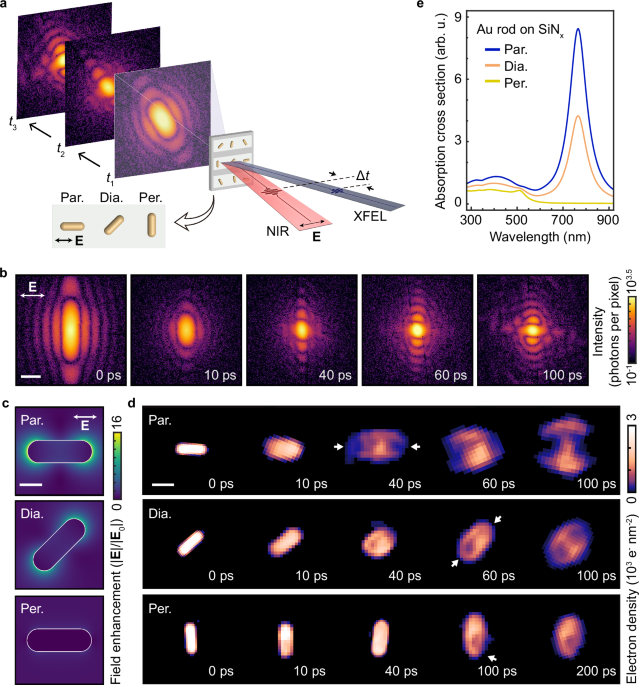
Unconjugated rod-shaped Au nanoparticles with a diameter of 50 nm and length of 145 nm, exhibiting peak surface plasmon resonance in the range of 800 nm (NanopartzTM), were mounted on 100 nm thin SiNx membranes. The membranes were custom designed (Silson LTD) with an array of multiple membranes, forming 36 × 2 arrays with individual membrane sizes of 9.0 mm × 0.2 mm, placed on a 25 mm × 25 mm frame. This design facilitated single-pulse diffraction experiments using a fixed-target sample delivery scheme33. To achieve a high particle hit rate, Au NRs in deionized purified water were spin-coated onto SiNx membranes, resulting in a nominal inter-particle distance of 3–5 μm. Single-pulse imaging experiments were conducted, ensuring one XFEL pulse per particle and one IR laser pulse in raster-scan mode. When the SiNx window was exposed to the IR laser pulse, it broke completely. To prevent laser-induced damage to neighboring particles, the shot-to-shot distance was set to 380 μm, greater than the laser footprint of x window remained intact. Each single pulse diffraction pattern was recorded on the multiport charge-coupled device detector with a pixel size of 50 μm by 50 μm34. The total detector area with 1024 by 1024 was used.
Coherent diffraction patterns, phase retrieval, and image reconstruction
Coherent single-pulse X-ray diffraction from individual Au nanorods was collected, and the sample was moved to a fresh particle after each exposure5. Diffraction patterns with multi-particle hits, identified by fringe spacing inconsistent with a single object, were discarded (Supplementary Fig. 2). Diffraction intensities were sampled finer than the Nyquist frequency set by the particle size to ensure accurate reconstruction35,36,37.
Real-space images were obtained from each single diffraction pattern by phase retrieval using iterative algorithms16,38. In each reconstruction cycle, the algorithm alternated between reciprocal and real space. The measured diffraction amplitudes were combined with an estimated phase and inverse Fourier transformed to produce a trial image. Real-space constraints were then applied to this image, including a finite support and positivity. The constrained image was Fourier transformed back to reciprocal space, where the calculated amplitudes were replaced with the measured values. Iterations were repeated until the reconstruction error stabilized. To ensure reliability, consistency was verified using multiple random starting phases for each pattern. For each pump-probe delay, a representative image that reflects the average response was selected from several independent reconstructions (Supplementary Movies 1–11).
Workflow for processing and reconstructing diffraction patterns
The diffraction patterns shown in Fig. 1b contained reconstructed pattern as the collected data has center part blocked by the detector. The raw diffraction data we acquired is shown as the “Raw pattern” in Supplementary Fig. 3a. The missing center caused by such beam stopper is retained within the central speckle to reconstruct the images from the measured, center missed data39. The processed pattern is then used to reconstruct the real-space image through iterative phase retrieval algorithms. The “Reconstructed pattern” in the third panel of Supplementary Fig. 3 represents the result after performing an inverse Fourier transform on the retrieved data. This reconstruction is subsequently used to fill the masked regions of the input pattern, yielding the “Filled pattern” shown in the fourth panel. This procedure ensures that the masked regions in the input data are addressed without introducing interpolation or artificial artifacts.
Orientation and aspect ratio determination for each Au NR
We used MATLAB’s regionprops function, which extracts geometric properties from binary images of particles. The centroid (geometric center) was calculated as the arithmetic mean of the pixel coordinates belonging to the particle, representing the average position of all pixels. Using the same function, we also obtained the major axis length (long axis), minor axis length (short axis), and the orientation. Based on this information, we categorized the orientations as Par. (parallel, 0–22.5°), Dia. (diagonal, 22.5°–67.5°), or Per. (perpendicular, 67.5°–112.5°) regarding to the laser polarization direction (Supplementary Fig. 4).
Near-field enhancement and absorption cross-section calculations
Numerical simulations of near-field enhancement for an Au NR on a SiNx substrate under linearly polarized electric fields were performed using BEM, as implemented in the MNPBEM-MATLAB toolbox developed by Hohenester and Trügler22. The BEM simulations were executed in retardation mode, modeling an Au NR with a 50 nm diameter and a total height of 145 nm, positioned above a 100 nm-thick SiNx substrate, matching experimental conditions (Supplementary Fig. 5a). The environment was vacuum, and the mesh discretization used 16, 8, and 15 elements for the azimuthal, polar, and longitudinal directions, respectively, with a total of 420 boundary elements. The complex refractive index of gold was taken from Johnson and Christy40, while SiNx was assigned a refractive index of 2, with the surrounding vacuum set to a refractive index of 1. Simulations were conducted for three different NR orientations, Par., Dia. and Per. by rotating the E-field polarization (0°, 45°, and 90°) while keeping the Au NR orientation fixed. The results include near-field cross-sections on the xy-plane (Fig. 1c), as well as cross-sections of xz-plane and z-projected averaged near-field distributions, shown in Supplementary Fig. 5b,c.
For the absorption cross-section spectra, the same simulation setup was used, with calculations performed over a wavelength range of 300 nm to 1200 nm.
Shape deformation rate quantification of the Au NRs
The shape deformation rate was obtained by fitting the temporal evolution of the aspect ratio to an exponential decay function described by the following equation:
$$y={a}_{1} * \exp \left(-\frac{t}{{\tau }_{1}}\right)+{b}_{1}$$
(1)
where \(y\) is the aspect ratio, \(t\) is the time delay, \({\tau }_{1}\) is the shape deformation time, \({a}_{1}\) is the initial amplitude, and \({b}_{1}\) is the converging aspect ratio. The fitting results for the shape deformation rate in different laser fluence (170, 230, 300, and 350 mJ cm−2) and orientations of the NR (parallel, diagonal, and perpendicular to the incident laser polarization direction) are summarized in the accompanying table and graph (Supplementary Table 1, Supplementary Fig. 6)
Scaling the shape deformation rate into one curve
We defined the scaled time as \({t}_{{{\rm{scaled}}}}=t\times (\frac{{E}_{{{\rm{eff}}}}}{{E}_{0}})\), where effective electric field \(({E}_{{{\rm{eff}}}}(\lambda,\varPhi,\theta ))\) is given by \({E}_{{{\rm{eff}}}}(\lambda,\varPhi,\theta )=\sqrt{\frac{u}{{{{\rm{\varepsilon }}}}_{0}}}\). Here, \(u\) is the absorbed energy density, determined as \(u=\frac{{\partial }_{{{\rm{abs}}}}\left(\lambda,\theta \right)\times F(\lambda,\varPhi,\theta )}{V}\), where \({\partial }_{{{\rm{abs}}}}(\lambda,\theta )\) is absorption cross-section, \(F(\lambda,\varPhi,\theta )\) is laser fluence at given \(\lambda\) (laser wavelength), \(\varPhi\) (laser fluence), and \(\theta\) (NR orientation) (see Supplementary Table 2). \(V\) is the volume of single Au NR with a diameter of 50 nm and a length of 145 nm. The reference electric field (\({E}_{0}\)) is the effective electric field for 800 nm, parallel polarization of 170 mJ cm−2 incidence fluence of the fastest reaction case in the low fluence shape-deformation mode.
To represent the shape deformation rate on a logarithmic scale, the aspect ratio was normalized using, \({{{\rm{AR}}}}_{{{\rm{scaled}}}}=({{\rm{AR}}}\left(\lambda,\varPhi,\theta \right)-{b}_{1}\left(\lambda,\varPhi,\theta \right))/{a}_{1}(\lambda,\varPhi,\theta )\) where AR is the aspect ratio of the NR, \({b}_{1}\) is the converging aspect ratio and \({a}_{1}\) is the amplitude of the aspect ratio from the shape deformation rate fit, at given \(\lambda,\varPhi,\theta\) (see Supplementary Table 1).
Characterization of the oscillatory behavior in the Au NRs
The expansion and oscillatory behavior in the temporal evolution of the long and short axis were analyzed by fitting the data using the following equation:
$$y={a}_{2} * \left[1-\exp \left(-\frac{t}{{\tau }_{2}}\right)\right]+{b}_{2}+A * \cos \left[\frac{2{{\rm{\pi }}}}{T}\left(t+{t}_{0}\right)\right],$$
(2)
where \(y\) is the scaled length, \(t\) is the time delay, \({\tau }_{2}\) is the characteristic time for expansion, \({a}_{2}\) is the amplitude of the exponential expansion, \({b}_{2}\) is the baseline length, A is the amplitude of the oscillation, T is the oscillation period, and \({t}_{0}\) is the phase shift. The fitting results for the oscillatory behavior observed in the low and high shape-deformation modes are summarized in the accompanying table (Supplementary Table 3).
To account for the eigenfrequency shift caused by shape deformation (AR decrease) during the energy-relaxation process for both low- and high-frequency modes, we tracked the temporal evolution of the aspect ratio and computed the corresponding eigenmodes (Supplementary Tables 4, 5). The period evolution was derived from the eigenfrequencies and modeled as a linear transition between the initial (pre-deformation) and final (post-deformation) states, expressed as \(f=\left(\frac{{T}_{{{\rm{end}}}}-{T}_{{{\rm{start}}}}}{{t}_{{{\rm{end}}}}-{t}_{{{\rm{start}}}}}\right)t+{T}_{{{\rm{start}}}}\), where \({T}_{{{\rm{start}}}}\) and \({T}_{{{\rm{end}}}}\) are the period before and after deformation, and \({t}_{{{\rm{start}}}}\) and \({t}_{{{\rm{end}}}}\) denote the time delays corresponding to 0 ps and the final time step, respectively.
This evolving eigenfrequency was incorporated into the oscillation equation, modifying the oscillation equation as follows:
$$y={a}_{2} * \left[1-\exp \left(-\frac{t}{{\tau }_{2}}\right)\right]+{b}_{2}+A * \cos \left[\frac{2{{\rm{\pi }}}}{\left(\frac{{T}_{{{\rm{end}}}}-{T}_{{{\rm{start}}}}}{{t}_{{{\rm{end}}}}-{t}_{{{\rm{start}}}}}\right)t+{T}_{{{\rm{start}}}}}\left(t+{t}_{0}\right)\right]$$
(3)
The dotted gray lines in Fig. 2d illustrate the eigenfrequency shift predicted by this model, showing how the frequency evolves dynamically with the changing NR morphology.
LSP mode calculations
Numerical simulations of the surface plasmon modes for the Au NR were performed using the BEM, as implemented in the MNPBEM toolbox22. The BEM simulation was initialized in quasistatic mode. The Au NR was modeled with a diameter of 50 nm and a total height of 145 nm, maintaining the same geometry as used in the near-field enhancement and absorption cross-section calculations.
The complex refractive index of gold from Johnson and Christy was employed, with the surrounding environment set to vacuum (refractive index of 1)39. The first 20 LSP eigenmodes were computed for the Au NRs and then excited with the incident light polarized along the NR’s long axis (Supplementary Fig. 8). Considering the amplitudes of each eigenmode, the LSP transverse modes were summed to construct the low absorption shape-deformation mode, while the LSP longitudinal modes were summed to construct the high-absorption shape-deformation mode41.
Displacement and stress field from acoustic distortion calculations
This simulation was performed using finite-element continuum modeling for the structural mechanics module/eigenfrequency solver in the three-dimensional finite-element software (COMSOL Multiphysics). The geometry of the Au NR was modeled as a hemispherical-capped cylinder with a diameter of 50 nm and length of \(\approx\)90 nm to match the intact Au NRs in our sample prior to shape deformation. To account for substrate effects, a 200 nm × 200 nm × 100 nm Si3N4 substrate was modeled beneath the Au NR.
The elastic moduli used for the Au NR were 70 GPa for low vibration modes, and 79 GPa for high vibration modes, with a Poisson’s ratio of 0.42 for both modes. The Si3N4 substrate was assigned an elastic modulus of 250 GPa and a Poisson’s ratio of 0.23.
We considered solid-type vibrations since the solid-to-liquid transition occurs due to vibrations originating from the solid state, and the phase remains partially solid during the initial stages of shape deformation.
TTMD simulations
MD simulations were conducted on an unsupported cylindrical gold rod, which was five times smaller than those used in experiments. After an initial equilibration at room temperature for 10 ps within a canonical ensemble, TTMD simulations were performed. Given that the sample geometry differed from the nanospheres used in refs. 5,6, the TTMD program was modified to accommodate cylindrical geometry. TTMD was used to describe the electron-ion nonequilibrium states by solving a heat diffusion equation as follows, \({C}_{{{\rm{e}}}}\frac{\partial {T}_{{{\rm{e}}}}}{\partial t}=\nabla \cdot \left({K}_{{{\rm{e}}}}\nabla {T}_{{{\rm{e}}}}\right)-G\left({T}_{{{\rm{e}}}}-{T}_{{{\rm{l}}}}\right)+S\left({{\bf{r}}},t\right)\). The parameters for electronic heat capacity (Ce), thermal conductivity (Ke), and electron-phonon coupling constant (G) were taken from ref. 5, where their temperature-dependent values were detailed.
The energy input, \(S\left({{\bf{r}}},t\right)={f}_{{{\rm{a}}}}\left({{\bf{r}}},t\right)\frac{{F}_{{{\rm{abs}}}}}{\tau {l}_{{{\rm{p}}}}}\sqrt{\frac{4{{\mathrm{ln}}}2}{{{\rm{\pi }}}}}\exp \left(-\frac{{r}_{0}-r}{{l}_{{{\rm{p}}}}}\right){{\mathrm{exp}}}\left[-\frac{4{{\mathrm{ln}}}(2){(t-{t}_{0})}^{2}}{{\tau }^{2}}\right]\) was modeled to account for the laser absorption, with parameters including absorbed fluence (Fabs), pulse width (\(\tau\)), and absorption length (\({l}_{{{\rm{p}}}}\)). Fabs = 80 mJ cm−2, \(\tau\) = 50 fs, \({l}_{{{\rm{p}}}}=25\) Å, and r0 = 50 Å were used. The anisotropy factor, \({f}_{{{\rm{a}}}}\left({{\bf{r}}},t\right)\), was introduced to account for plasmonic excitation effects, distinguishing between transverse and longitudinal plasmonic modes. These modes were described using spatial and temporal dependencies, ensuring accurate representation of plasmonic field enhancement. The normalization constant and the field enhancement factors were chosen to replicate the experimental conditions, with symmetry considerations for transverse and longitudinal excitations.
$${f}_{{{\rm{a}}}}^{{{\rm{trans}}}}\left({{\bf{r}}},t\right)=\left\{\begin{array}{c}{\alpha }_{1}A\exp \left(\frac{r-{r}_{0}}{{r}_{0}}\right)\exp \left(-\frac{\left|z-{cH}\right|}{{cH}}\right)\left|\cos \varphi \right|\left|\cos \left(\frac{t}{T}\right)\right|\quad\left(0\le z\right)\\ {\alpha }_{2}A\exp \left(\frac{r-{r}_{0}}{{r}_{0}}\right)\exp \left(-\frac{\left|z+{cH}\right|}{{cH}}\right)\left|\cos \varphi \right|\left|\sin \left(\frac{t}{T}\right)\right|\quad\left(z
(4)
$${f}_{{{\rm{a}}}}^{{{\rm{long}}}}\left({{\bf{r}}},t\right)=\left\{\begin{array}{c}{\alpha }_{1}A\exp \left(\frac{r-{r}_{0}}{{r}_{0}}\right)\exp \left(-\frac{\left|z-{cH}\right|}{{cH}}\right)\left|\cos \left(\frac{t}{T}\right)\right|\quad\left(0\le z\right)\\ {\alpha }_{2}A\exp \left(\frac{r-{r}_{0}}{{r}_{0}}\right)\exp \left(-\frac{\left|z+{cH}\right|}{{cH}}\right)\left|\sin \left(\frac{t}{T}\right)\right|\quad\left(z
(5)
The normalization constant of A = 0.043, the cylinder height of H = 286 Å and a plasmonic frequency of T = 0.45 fs were used. \(\varphi\) is an azimuthal angle. The field enhance factor of \({\alpha }_{1}={\alpha }_{2}=16\) were used for transverse mode, and \({\alpha }_{1}=16,{\alpha }_{2}=1\) for longitudinal mode. \(c=0.2\) and \(0.5\) were used for the transverse and longitudinal modes, respectively.