1. Introduction
In critical engineering applications such as subsonic transport aircraft, skin friction drag strongly depends on the state of the boundary layer (i.e. laminar or turbulent) developing on main wings and stabilisers. The considerable contribution of skin friction drag to the total aerodynamic drag can be reduced by either manipulating the turbulent boundary layer resulting from laminar–turbulent transition or by delaying the onset of transition, i.e. through laminar flow control (LFC) (Arnal Reference Arnal1996). The use of LFC showed promise in both laboratory studies and flight tests (Joslin Reference Joslin1998) and largely motivates the present work. However, the effectiveness of LFC is known to be hindered by structural and geometrical imperfections present on realistic wings, such as steps, gaps or grooves, that affect the boundary layer transition process (Wang & Gaster Reference Wang and Gaster2005; Crouch, Kosorygin & Ng Reference Crouch, Kosorygin and Ng2006). Such imperfections arise due to manufacturing tolerances as well as operational wear and tear (Worner, Rist & Wagner Reference Worner, Rist and Wagner2003). Various studies have found that steps (Rius-Vidales & Kotsonis Reference Rius-Vidales and Kotsonis2020; Casacuberta et al. Reference Casacuberta, Hickel, Westerbeek and Kotsonis2022), gaps (Forte et al. Reference Forte, Perraud, Séraudie, Beguet and Casalis2015), waviness (Holmes et al. Reference Holmes, Obara, Martin and Domack1985; Westerbeek & Kotsonis Reference Westerbeek and Kotsonis2022) and humps (Franco Sumariva, Hein & Valero Reference Franco Sumariva, Hein and Valero2020) alter the stability of the boundary layer and are a source of laminar flow deterioration (i.e. the transition front is moved upstream, thus reducing the extent of laminar flow). The flow behaviour and eventual transition scenario vary with the type of instability interacting with the aforementioned surface imperfections.
Swept wings are a key focus area for LFC, inasmuch as they are widely used in subsonic transport aircraft. The laminar–turbulent transition of subsonic boundary layers over swept wings is driven by the growth of four distinct instability types; namely Görtler vortices, attachment line instabilities, Tollmien–Schlichting (TS) waves and cross-flow instability (CFI). The Görtler instability arises due to concave surface curvature and is commonly controlled through opportune wing profile design (Reed & Saric Reference Reed and Saric2002). The leading-edge attachment line has been observed to be unstable to viscous Tollmien–Schlichting-like waves as found in Blasius flow (Theofilis Reference Theofilis1998). A reduced leading-edge curvature can mitigate the attachment line instability. Consequently, the most critical instability kinds in swept wing flow are Tollmien–Schlichting waves and CFI (Saric, Reed & White Reference Saric, Reed and White2003). The latter may manifest in either stationary or travelling form; see Deyhle & Bippes (Reference Deyhle and Bippes1996) for a discussion on pertinent receptivity mechanisms. Swept wing boundary layers typically experience significant growth of stationary CFI near the leading edge. These instabilities are generally responsible for transition in environments of low free stream turbulence (Deyhle & Bippes Reference Deyhle and Bippes1996; Downs & White Reference Downs and White2013) and are strongly destabilised under favourable pressure gradients (Bippes Reference Bippes1999). If transition is not anticipated due to CFI growth and the favourable pressure gradient is not maintained, the growth of TS waves can lead to transition further downstream in the mid-chord region (Reed & Saric Reference Reed and Saric1989).
1.1. Interaction between boundary layer instabilities and surface imperfections
Two-dimensional, i.e. invariant in one spatial direction, surface imperfections are commonly found to promote transition governed by TS instability (see for instance Nayfeh Reference Nayfeh1992; Masad & Iyer Reference Masad and Iyer1994; Perraud & Seraudie Reference Perraud and Seraudie2000 and Worner et al. Reference Worner, Rist and Wagner2003). Gao, Park & Park (Reference Gao, Park and Park2011) used the parabolised stability equations (PSE) method to study the interaction between incoming TS waves and a smooth hump, and found significant instability growth downstream of the hump. The main hump shape prevented the local formation of recirculating flow potentially giving rise to a global instability mechanism (Xu, Lombard & Sherwin Reference Xu, Lombard and Sherwin2017). However, for additional variations of the hump shape, the effects of the induced adverse pressure gradient and flow separation contribute to the destabilising influence of the hump. Park & Park (Reference Park and Park2013) carried out a similar analysis accounting for nonlinear perturbation effects. They described that the hump promotes instability growth even for perturbations with a small initial amplitude. Furthermore, it was noted that the amplitude of the incoming perturbation conditions the secondary instability growth more prominently than the shape of the hump. Franco Sumariva et al. (Reference Franco Sumariva, Hein and Valero2020) used the adaptive harmonic linearised Navier–Stokes (AHLNS) method to investigate the effect of two-dimensional humps that are either smooth or rectangular (i.e. a combination of forward- and backward-facing steps). They reported an increase in the perturbations amplitude downstream of the hump that is proportional to the height of the hump. Moreover, they found that the shape of the hump, i.e. smooth or rectangular, becomes increasingly important when the hump is of greater height.
It has been widely reported that the shape of the surface feature critically conditions the mechanisms of perturbation interaction and transition advancement. For instance, forward-facing steps (FFS) are less critical than backward-facing steps (BFS) in promoting transition (Perraud & Seraudie Reference Perraud and Seraudie2000; Wang & Gaster Reference Wang and Gaster2005; Crouch et al. Reference Crouch, Kosorygin and Ng2006). At the same certain conditions, FFS have the potential to stabilise incoming TS instability, for instance in the direct numerical simulation (DNS) by Worner et al. (Reference Worner, Rist and Wagner2003). To further investigate the mechanisms of TS wave stabilisation by an FFS, Barahona et al. (Reference Barahona, Rius-Vidales, Tocci, Ziegler, Hein and Kotsonis2022) combined experimental and numerical techniques to assess the interaction of a monochromatic (i.e. single frequency) TS wave with an FFS. Barahona et al. (Reference Barahona, Rius-Vidales, Tocci, Ziegler, Hein and Kotsonis2022) hypothesise that the Orr mechanism (Åkervik et al. Reference Åkervik, Ehrenstein, Gallaire and Henningson2008) is governing the perturbation evolution locally at the FFS.
Wu & Hogg (Reference Wu and Hogg2006) argued that incoming TS waves interacting with a localised surface feature are scattered due to the rapid spatial distortion of the base flow around the feature. The effect of the surface feature on the instability amplitude is quantified through a so-called transmission coefficient. Xu et al. (Reference Xu, Sherwin, Hall and Wu2016) further investigated the behaviour of incoming TS waves interacting with rapid localised base-flow distortions (

$\lt \mathcal{O}(\lambda _x)$
, i.e. smaller than the streamwise wavelength of the perturbation). Here, the earlier hypothesised linear dependence of amplification on the surface feature height could not be reconciled by small humps and indentations both destabilising incoming TS waves. Moreover, earlier statements by Wu & Hogg (Reference Wu and Hogg2006) of surface protuberances locally increasing the disturbance amplitude are nuanced by the finding that the effect occurs over a longer streamwise extent than the protuberance itself, indicating that some effects need not be localised.
Similar to TS waves, the interaction of CFI with forward- and backward-facing steps has been studied in detail. Both experimental and numerical studies found that the incoming cross-flow instabilities experience a wall-normal diversion as they approach the step, essentially being transported in the direction of the local mean flow streamlines. Meanwhile, the wall-normal perturbation velocity component shows a distinct secondary peak near the wall (Tufts et al. Reference Tufts, Reed, Crawford, Duncan and Saric2017; Eppink et al. Reference Eppink, Wlezien, King and Choudhari2018; Eppink Reference Eppink2020; Casacuberta, Hickel & Kotsonis Reference Casacuberta, Hickel and Kotsonis2021) and shortly downstream of the step corner, near-wall vortical structures arise (Eppink et al. Reference Eppink, Wlezien, King and Choudhari2018; Eppink Reference Eppink2020; Casacuberta et al. Reference Casacuberta, Hickel and Kotsonis2021; Rius-Vidales & Kotsonis Reference Rius-Vidales and Kotsonis2021). Casacuberta et al. (Reference Casacuberta, Hickel, Westerbeek and Kotsonis2022) demonstrated that numerical solutions of the nonlinear parabolised stability equations (NPSE) initiated from DNS data in the immediate proximity of the step were unsuccessful. However, when the initialisation point was displaced marginally downstream, close alignment with DNS outcomes was achieved. This observation was instrumental in establishing the non-modal characteristics inherent in the instability development in the immediate proximity of the step. Furthermore, a detailed examination of the near-wall vortical structures concluded that these structures may be influenced by the original incoming cross-flow instability, yet exhibit autonomous behaviour distinct from it (Casacuberta et al. Reference Casacuberta, Westerbeek, Franco, Groot, Hickel, Hein and Kotsonis2025).
In contrast to sharp surface modifications such as steps, the existing body of literature pertaining to the interaction between CFI and smooth surface modifications, such as humps, is limited. Cooke et al. (Reference Cooke, Mughal, Sherwin, Ashworth and Rolston2019) numerically investigated the interaction of both stationary and travelling CFI with localised bumps (i.e. a rapid succession of a smoothed forward- and backward-facing steps). They employed both linear harmonic Navier–Stokes (LHNS) and linear parabolised stability equation (LPSE) frameworks but found the LPSE to be incapable of providing accurate results. The presence of surface features generally proved destabilising for the incoming instabilities. However, in two scenarios where the bump height is low, travelling cross-flow instabilities were found to undergo stabilisation. Westerbeek et al. (Reference Westerbeek, Franco Sumariva, Michelis, Hein and Kotsonis2023) performed linear and nonlinear simulations of the interaction between stationary CFI and large aspect-ratio (i.e. width/height

${\gt } 50$
) smooth humps of varying height and width that featured no recirculation regions. They observed a consistent stabilisation of the fundamental mode of cross-flow instability, defined as the most unstable mode in the baseline case (i.e. no hump present). Higher harmonics were instead consistently destabilised by the hump. Both behaviours were found to be governed by linear production mechanisms.
More recently, motivated by the numerical work of Westerbeek et al. (Reference Westerbeek, Franco Sumariva, Michelis, Hein and Kotsonis2023), Rius-Vidales et al. (Reference Rius-Vidales, Morais, Westerbeek, Casacuberta, Soyler and Kotsonis2025) performed an exploratory proof-of-concept wind tunnel experiment, where a single smooth hump was installed on a

$45^{\circ }$
swept wing and tested at chord Reynolds number of approximately 2 million. The outcomes pointed to two distinct scenarios, notably influenced by the amplitude of incoming CFI. Specifically, compared with reference no-hump conditions, the hump was found to stabilise relatively low-amplitude incoming stationary CFI at a linear growth stage, and produced a significant extension of laminar flow of approximately 14 % of chord length. In contrast, when the incoming CFI was at relatively high amplitude and undergoing nonlinear growth, the hump was found to cause an abrupt transition advancement, essentially tripping the flow.
The majority of aforementioned studies treated the effect of single smooth surface modifications on boundary layer stability. However, plate rolling techniques and wing bending can lead to the formation of multiple and successive smooth surface modifications, which can be generalised as surface waviness in wings and profoundly affect the transition scenario (Nayfeh, Ragab & Al-Maaitah Reference Nayfeh, Ragab and Al-Maaitah1988). The effect of waviness on CFI has received some, but limited, attention. Masad (Reference Masad1996) found that the presence of surface undulations resulted in a destabilising effect on incoming cross-flow instabilities. Moreover, this effect was positively correlated to the undulation amplitude. Thomas et al. (Reference Thomas, Mughal, Gipon, Ashworth and Martinez-Cava2016) instead found a scenario that led to the stabilisation of the dominant CFI mode, but cited a sensitivity to undulation wavelength and phase with respect to the incoming mode. Lastly, Westerbeek & Kotsonis (Reference Westerbeek and Kotsonis2022) performed a numerical investigation into the effect of surface undulation shape on the nonlinear amplitude development of CFI, but found the effect of the undulation shape to be minor for the studied cases. The presence of undulations yielded a destabilising effect on the perturbations. This is in contrast to the positive effects of single smooth surface protuberances reported by Westerbeek et al. (Reference Westerbeek, Franco Sumariva, Michelis, Hein and Kotsonis2023). The negative effects of surface waviness were likely caused by the proximity of shape repetition, since Westerbeek et al. (Reference Westerbeek, Franco Sumariva, Michelis, Hein and Kotsonis2023) found stabilisation to occur significantly downstream of the single surface modification.
1.2. Use of smooth surface humps as a laminar flow control method
The recent observations by Westerbeek et al. (Reference Westerbeek, Franco Sumariva, Michelis, Hein and Kotsonis2023) and Rius-Vidales et al. (Reference Rius-Vidales, Morais, Westerbeek, Casacuberta, Soyler and Kotsonis2025) suggest the potential of smooth surface modifications, such as humps, as a practically feasible passive LFC method, in the specific use-case of swept wings. Preliminary results identified the robustness of the stabilisation to variations of chord Reynolds number, perturbation forcing conditions and pressure gradient (i.e. angle of attack). Under the effect of such a hump, the incoming stationary cross-flow instability is shown to undergo a series of stabilising and destabilising events that take place mostly downstream of the hump apex. The stabilisation is often found to be stronger than the preceding destabilisation, resulting in a downstream amplitude that is lower than in the clean reference case. Additionally, in cases where the transition location is advanced, higher harmonics appear to play an important role (Rius-Vidales et al. Reference Rius-Vidales, Morais, Westerbeek, Casacuberta, Soyler and Kotsonis2025). Nonlinear simulations of CFI interacting with a smooth hump by Westerbeek et al. (Reference Westerbeek, Franco Sumariva, Michelis, Hein and Kotsonis2023) showed a consistent destabilisation of higher harmonics. Despite these preliminary observations, the details of the underlying mechanism of interaction between the incoming CFI and the hump are still largely unknown. Specifically, the importance of incoming instability amplitude needs to be systematically tested to gain more insight into the (nonlinear) flow dynamics.
Navigating the large parameter space relating to the surface modification (size, shape, location, etc.), boundary layer characteristics and incoming instabilities (wavenumber, frequency, amplitude, etc.) requires a numerically efficient yet accurate approach. The effect of surface imperfections is often measured by considering the direct effect on transition location. In a wealth of past works, universal roughness-based Reynolds number thresholds were sought, above which surface features promote transition (see e.g. Holmes et al. Reference Holmes, Obara, Martin and Domack1985; Wang & Gaster Reference Wang and Gaster2005; Tufts et al. Reference Tufts, Reed, Crawford, Duncan and Saric2017). Alternatively, reduced-order models resort to finding a correction to the integral amplification factor (i.e.

$\Delta N$
-factor) based on surface features (see Crouch et al. Reference Crouch, Kosorygin and Ng2006; Crouch & Kosorygin Reference Crouch and Kosorygin2020). A linear numerical study by Edelmann & Rist (Reference Edelmann and Rist2014) found that streamwise position, step location, step height and Mach number affect the N-factor. However, as the

$\Delta N$
-factor method is linear per definition, the effect of perturbation amplitude is generally ignored. Indeed, both Eppink (Reference Eppink2020) and Rius-Vidales & Kotsonis (Reference Rius-Vidales and Kotsonis2020) noted that single-parameter models neglect key aspects of the underlying physics such as the incoming perturbation amplitude. These can be conditionally extracted in experiments or high-fidelity simulations. However, detailed parametric studies of the interaction between surface modifications and incoming instabilities are hindered in experiments by measurement limitations (noise, field of view, reach and intrusion) near the surface and numerically by the large computational costs involved with running transitional DNS. For those reasons, few studies are concerned with the effect of the incoming perturbation amplitude on the interaction with surface modifications at the scale of the boundary layer instabilities. Weakly nonlinear stability theory, as shown by e.g. Wu (Reference Wu2019), could be applied to perform stability calculations more efficiently. However, weakly nonlinear theories require a hierarchical ordering of the terms based on amplitude (Bertolotti, Herbert & Spalart Reference Bertolotti, Herbert and Spalart1992). Since this hierarchy is not generally known a priori, at least for the presently investigated flows, its application may not be valid for all inflow amplitudes. To prevent the weakly nonlinear assumption from affecting the analysis, a fully nonlinear framework is used here instead. In summary, the limitations of both traditional numerical and experimental approaches in tackling the interaction of boundary layer instabilities with surface modifications motivated the development of an efficient harmonic Navier–Stokes (HNS) framework as used in the present work (Westerbeek et al. Reference Westerbeek, Hulshoff, Schuttelaars and Kotsonis2024).
1.3. Aim and overview of the present work
The effect of smooth surface modifications, such as humps, on laminar–turbulent transition appears to be influenced largely by the amplitude of incoming disturbances, as demonstrated by the experiments of Rius-Vidales et al. (Reference Rius-Vidales, Morais, Westerbeek, Casacuberta, Soyler and Kotsonis2025). The present work aims to improve understanding of the stabilising and/or destabilising effect of smooth surface humps on incoming CFI, further enabling the design of such geometries as a realisable and practical passive LFC method. To elucidate these effects, a parametric sweep of the amplitude of the incoming CFI is deployed based on harmonic Navier–Stokes simulations. A stability and energy budget examination is conducted to assess how certain hump-induced base flow features, e.g. changes of the base flow profiles, inflection points, cross-flow reversal or local pressure gradients, qualitatively and quantitatively influence the development of the incoming CFI.
The work is structured as follows. The methodology is outlined in § 2. Herein, the domain and flow cases are described, followed by a presentation of the techniques used for extracting the base flow, perturbation development and energy budget. The topology of the base flow is scrutinised in § 3, while in § 4, the nonlinear interaction of incoming CFI with varying amplitude and the hump is analysed. Local linear stability frameworks are also leveraged for this analysis.
2. Methodology
In this work, the geometry of the hump and the flow conditions are guided by the experiments of Rius-Vidales et al. (Reference Rius-Vidales, Morais, Westerbeek, Casacuberta, Soyler and Kotsonis2025), which provided evidence of transition delay of approximately 14 % chord length by a surface hump in CFI-dominated flow, when the incoming CFI was intercepting the hump at relatively low amplitude. The observed transition delay was found to be robust to changes in the Reynolds number. However, when the incoming CFI was at a higher amplitude, the hump was found to promote early transition (i.e. the transition front is shifted upstream when compared with reference no-hump conditions). In these experiments, the amplitude of incoming CFI was controlled via the height of micrometric discrete roughness elements (DREs) located near the wing leading edge, see for instance Zoppini et al. (Reference Zoppini, Westerbeek, Ragni and Kotsonis2022).
In the present work, mechanisms of unsteady instability and laminar breakdown are not accounted for in the numerical simulations. The goal of this work is particularly placed on the characterisation of the effects of the initial CFI amplitude on the mechanisms of stationary perturbation growth and decay due to the hump. The truncation of the flow to the dominant stationary spectral components of the instability system thus greatly simplifies the computational complexity and resource demand. By the assumption that transition is driven by the amplification of classic modal primary and secondary CFI instabilities (i.e. path A in the Reshotko/Morkovin map Reshotko & Tumin Reference Reshotko and Tumin2006), the growth behaviour and amplitude of the primary instability are used as proxies of laminar–turbulent transition.
2.1. Flow conditions and domain geometry
All quantities in this work will be shown in non-dimensional form unless specified. Dimensional quantities are denoted with an overbar. Global characteristic scales are used to non-dimensionalise the equations due to the non-local nature of the HNS framework used in this work. The reference length
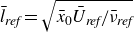
$\bar {l}_{\textit{ref}}=\sqrt {{\bar {x}_0 \bar {U}_{\textit{ref}}}/{\bar {\nu }_{\textit{ref}}}}$
is defined as the Blasius length scale at the inflow of the numerical domain, i.e. at

$\bar {x} = \bar {x}_0$
(see figure 1). The reference kinematic viscosity is denoted as

$\bar {\nu }_{\textit{ref}}$
and all velocity quantities are normalised by the reference velocity

$\bar {U}_{\textit{ref}}$
, taken as the external (i.e. inviscid free stream) chordwise (i.e. pointing in the direction orthogonal to the leading edge,

$x$
) velocity at the simulation domain inflow. The Reynolds number is defined as
$\textit{Re} = {\bar {l}_{\textit{ref}} \bar {U}_{\textit{ref}}}/{\bar {\nu }_{\textit{ref}}}$
. The reference values used in the present work are summarised in table 1.
Table 1. Reference quantities used in the present work.
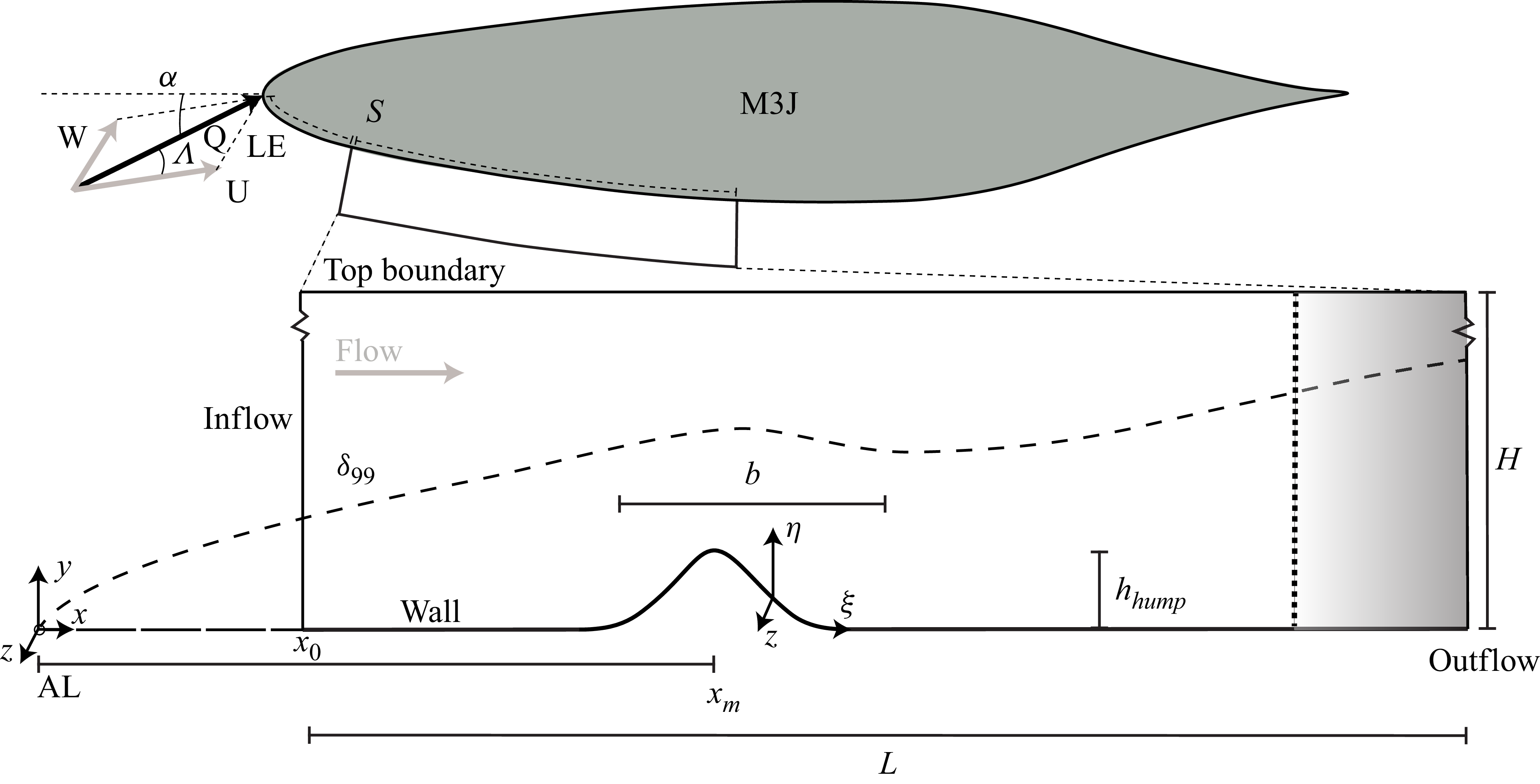
The experiments of Rius-Vidales et al. (Reference Rius-Vidales, Morais, Westerbeek, Casacuberta, Soyler and Kotsonis2025) were performed on the M3J swept-wing model featuring a symmetric aerofoil and a

$45^{\circ }$
sweep angle. The maximum profile thickness is placed at 65 % chord to maintain a favourable pressure gradient over a large chordwise extent. Measurements were performed on the pressure side of the wing and at an angle of attack,

$\alpha$
, of

$3^{\circ }$
. This ensures favourable conditions for the growth of cross-flow instabilities while suppressing other types of instabilities such as Tollmien–Schlichting waves and Görtler vortices. For a detailed description of the wing design, the reader is referred to Serpieri & Kotsonis (Reference Serpieri and Kotsonis2016). Stationary CFI was introduced via DREs placed at a distance of 2.5 % of chord from the leading edge. The resulting perturbation is shown to trigger the most unstable mode for the considered domain and is characterised by the angular frequency

$\omega _1=0$
(i.e. a stationary mode) and the spanwise wavenumber
$\beta _1 = 2\pi / \lambda _z = 0.1831$
, where

$\lambda _z$
denotes the spanwise wavelength. The subscript

$1$
refers to the fundamental component of the truncated Fourier series. This notation is employed here due to the use of a nonlinear stability framework, as outlined in § 2.3. The DRE height in the experiments is adjusted to introduce CFI at varying amplitudes (Zoppini et al. Reference Zoppini, Westerbeek, Ragni and Kotsonis2022) which is modelled in the present simulations by imposing the inflow amplitude and shape of the fundamental mode

$(0,1)$
directly. The treatment of the inflow boundary is covered in more detail in § 2.3.
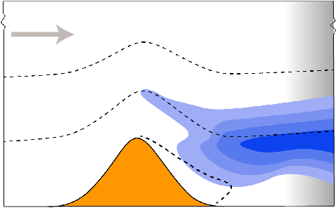
In the wind tunnel measurements of Rius-Vidales et al. (Reference Rius-Vidales, Morais, Westerbeek, Casacuberta, Soyler and Kotsonis2025), the local aerofoil curvature at the location of the hump is orders of magnitude smaller than the curvature of the hump and hence it is neglected for the purpose of this investigation. The flow problem correspondingly considers a rectangular domain containing an inflow boundary, a top boundary, a wall featuring the smooth hump and an outflow boundary (see figure 1). A global Cartesian coordinate system is considered, denoted by

$(x,y,z)$
, with

$x$
indicating the direction orthogonal to the leading edge and

$z$
is the direction parallel to the leading edge. The direction

$y$
completes the coordinate system. The numerical coordinates read

$(\xi ,\eta ,z)$
with the

$\xi$
-axis pointing orthogonal to the leading edge, but following the surface hump, in a body-fitted sense. The hump shape is given approximately by
(2.1)
\begin{align} y(x) = h \; \textrm {exp}\!\left (0.5\left (\frac {x-618.96}{37.7}\right )^2 \right )\!, \end{align}
where all parameters are non-dimensionalised with the reference length (

$\bar {l}_{\textit{ref}}$
). The resulting hump has a width
$b =229 \equiv 0.056 \bar {c}$
and a height

$h =4.58$
, thus

$b/h = 50$
. The hump is symmetrical around its centre, which is located at
$x_m\ (\equiv 619 \bar {l}_{\textit{ref}}= 0.15 \bar {c}$
), relative to the attachment line (AL). The

$\eta$
-axis is offset by the surface hump, though it remains parallel to the

$y$
-axis (see figure 1). The perturbation equations are numerically solved in the aforementioned domain in the (

$\xi ,\eta ,z$
) coordinates via a coordinate transformation from the Cartesian coordinate system, (

$x,y,z$
). The

$u$
-,

$v$
– and

$w$
-velocity components are defined in the direction of

$x$
,

$y$
and

$z$
, respectively. The perturbation kinetic energy is defined as
$E_k = \sqrt {u^{\prime \; 2} + v^{\prime \; 2} + w^{\prime \; 2}}$
, where the prime indicates perturbation quantity.
The inflow boundary of the numerical domain,

$x = x_0 = 214$
, corresponds virtually to 5 % of the chord of the reference wing and is located at a distance of

$214$

$\bar {l}_{\textit{ref}}$

$(= 0.05 \bar {c}$
, where

$\bar {c}=0.9$
m) reference lengths downstream of the effective AL. The chordwise length of the domain is
$L = 1156\ (\equiv 0.28 \bar {c}$
) and the height of the numerical domain is

$H =91$
, equivalent to

$27\delta _{99}$
at the inflow. The choice of domain height was based on the typical compromise between accuracy and numerical efficiency. The chosen value was taken through a sensitivity study and was based on solution invariance with domain height, while maintaining a sufficiently fine grid spacing.
2.2. Base flow calculation
The numerical framework for stability analysis in this work is based on the perturbation equations which require a pre-calculated solution of the unperturbed base flow. To this end, computations of the incompressible base flow are carried out independently by use of the commercial finite-element solver COMSOL. The set-up features a square domain discretised in second-order elements for velocities and first-order elements for pressure. In the wall-normal direction,

$96$
elements were present, which are clustered near the wall with an exponential function. In the chordwise direction,

$1320$
elements were present with additional refinement around the hump. By virtue of spanwise invariance in the base flow, only two elements were considered in the

$z$
-direction.
2.2.1. Base flow boundary conditions
The boundary conditions used in the computations of the base flow are described next. For both hump and reference cases, the static pressure at the top boundary of the base flow domain is prescribed and set to be identical to the pressure measured in the experiments of Rius-Vidales et al. (Reference Rius-Vidales, Morais, Westerbeek, Casacuberta, Soyler and Kotsonis2025) on the wing surface at reference no-hump conditions. The validity of this boundary condition for the current domain and wing was confirmed via complimentary Reynolds-averaged Navier–Stokes (RANS) simulations of the wind tunnel experiments of Rius-Vidales et al. (Reference Rius-Vidales, Morais, Westerbeek, Casacuberta, Soyler and Kotsonis2025). (Simulations performed by Mohammad Moripiri and Ardeshir Hanifi, KTH, Sweden.) The simulations showed a strong similarity between the static wall pressure and the static pressure at a surface orthogonal distance of H ( = 91

$l_{\textit{ref}}$
) away from the wing surface. The pressure imposed at the top boundary results in an external (i.e. inviscid) velocity distribution as described by Casacuberta et al. (Reference Casacuberta, Hickel, Westerbeek and Kotsonis2022, (2.14)). Additionally, second-order wall-normal velocity derivatives were suppressed at the top boundary. This accommodates the presence of a streamwise pressure gradient which results in non-zero first-order wall-normal derivatives for velocities at the top boundary. Lastly, a constant external spanwise velocity,
$\bar {W}_e= -1.35 \bar {U}_{\textit{ref}}$
, was prescribed at the top boundary, to model the swept flow conditions.
The solution to the Falkner–Skan–Cooke equation corresponding to the local pressure gradient was imposed at the inflow, in conjunction with a first-order Neumann condition for the pressure. At the outflow, static pressure is prescribed equal to the static pressure at the top boundary at the corresponding

$x$
location. At the wall, the no-slip and no-penetration conditions are enforced. Periodic boundary conditions are imposed in the transverse boundaries.
2.3. Flow stability simulation
The in-house solver for nonlinear HNS, DeHNSSo, is employed to compute numerical solutions of the perturbation equations. The reader is referred to Westerbeek et al. (Reference Westerbeek, Hulshoff, Schuttelaars and Kotsonis2024) for details on the HNS method and the numerical framework. The unsteady incompressible Navier–Stokes equations are considered, which in non-dimensional form read as
(2.2a)
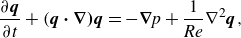
\begin{align} \frac {\partial \boldsymbol{q}}{\partial t} + ( \boldsymbol{q} \boldsymbol{\cdot } \boldsymbol{\nabla )}\boldsymbol{q} &= – \boldsymbol{\nabla \!} p + \frac {1}{\textit{Re}}{\nabla }^2 \boldsymbol{q}, \end{align}
(2.2b)

\begin{align} \boldsymbol{\nabla } \boldsymbol{\cdot } \boldsymbol{q} &= 0. \end{align}
The

$p$
is the static pressure and the velocity vector

$\boldsymbol{q}=[u \; v \; w]^T$
expresses the total flow, i.e. the superposition of base flow,

$\boldsymbol{Q}$
, and perturbation fields,

$\boldsymbol{q}’$
, such that
(2.3)

\begin{equation} \boldsymbol{q}(\xi ,\eta ,z,t) = \boldsymbol{Q}(\xi ,\eta ) + \boldsymbol{q}'(\xi ,\eta ,z,t), \end{equation}
where

$\boldsymbol{q’}$
assumes a harmonic expansion along the

$z$
-axis and in time

$t$
.
On introducing (2.3) into (2.2) and removing the base-flow equation, the perturbation equations are obtained, as
(2.4a)

\begin{align} \frac {\partial \boldsymbol{q’}}{\partial t} + (\boldsymbol{Q} \boldsymbol{\cdot } \boldsymbol{\nabla }) \boldsymbol{q’} + (\boldsymbol{q’} \boldsymbol{\cdot } \boldsymbol{\nabla }) \boldsymbol{Q} + (\boldsymbol{q’} \boldsymbol{\cdot } \boldsymbol{\nabla }) \boldsymbol{q’} &= -\boldsymbol{\nabla \!} p’ + \frac {1}{Re}{\boldsymbol{\nabla}}^2 \boldsymbol{q’}, \end{align}
(2.4b)

\begin{align} \boldsymbol{\nabla } \boldsymbol{\cdot } \boldsymbol{q’} &= 0. \end{align}
Finally, the perturbation field is expressed as a truncated Fourier series, i.e.
(2.5)
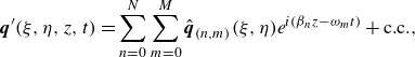
\begin{equation} \boldsymbol{q}'(\xi ,\eta ,z,t) = \sum _{n=0}^N \sum _{m=0}^M\hat {\boldsymbol{q}}_{(n,m)}(\xi ,\eta ) e^{{i}(\beta _n z – \omega _m t)} + \textrm {c.c.}, \end{equation}
and introduced into (2.4), where

$\omega \in \mathbb{R}$
, and

${i}^2 = -1$
. The moduli of

$\hat {\boldsymbol{q}}_{(n,m)} \in \mathbb{C}$
will be referred to as the amplitude functions, the fundamental spanwise mode is denoted by

$\beta _1$
and the c.c. expresses the complex conjugate. The non-oscillatory perturbation, or so-called mean flow distortion (MFD), corresponds to
$(m,n)=(0,0)$
. In the present nonlinear simulations, higher-order harmonics and the mean-flow distortion are allowed to rise by modal interactions up to

$N=5$
downstream of the inflow, and only stationary modes are considered (i.e.

$M=0$
). The

$N\gt 5$
harmonic modes are disregarded from the numerical simulations, inasmuch as an order of magnitude analysis suggests that they contribute no more than 0.42 % to the total perturbation kinetic energy for any of the considered cases.
In contrast to classical stability methods such as PSE, the HNS formulation does not make use of a spatial wavenumber in the perturbation ansatz of (2.5), as all spatial growth and oscillatory motion is enclosed in the amplitude function

$\hat {\boldsymbol{q}}_{(n,m)}$
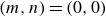
. Nevertheless, the evaluation a posteriori of growth-rate metrics is instructive for the analysis and interpretation of results. Here, growth rate is computed as
(2.6)
\begin{equation} \alpha _{i} = -\frac {1}{|f’_{(m,n)}|} \frac {{\rm d} |f’_{(m,n)}|}{\textrm {d} x}, \end{equation}
with

$|f’_{(m,n)}|$
measured at a chosen wall-normal location. Due to the ability of the HNS framework to simulate the development of modal or non-modal perturbations in fully non-parallel flows, the choice of perturbation quantity

$f’$
has an effect on the value of the resulting growth rate. In this work, the maximum amplitude of chordwise perturbation velocity

$|u’|$
and the wall-normal integral of perturbation kinetic energy are used as perturbation quantities

$f’$
.
2.3.1. Perturbation boundary conditions
The boundary conditions for the HNS simulations are discussed here briefly for completeness, although a more in-depth overview of the implementation can be found from Westerbeek et al. (Reference Westerbeek, Hulshoff, Schuttelaars and Kotsonis2024). A non-homogeneous Dirichlet condition is used at the inflow, namely, the solution to the local Orr–Sommerfeld (OS) eigenvalue problem considering

$\beta = \beta _{1}$
. The perturbation profile is normalised and the desired inflow amplitude is assigned to it. All additional modes of the truncated Fourier series (2.5) are initiated with a zero amplitude and arise naturally further downstream as a result of nonlinear interactions. The spanwise wavelength and the range of investigated inflow amplitudes of the inflow mode are chosen to respectively match the spanwise spacing of DREs in the experiments of Rius-Vidales et al. (Reference Rius-Vidales, Morais, Westerbeek, Casacuberta, Soyler and Kotsonis2025) (

$\bar {\lambda }_{\textit{DRE}}$
= 7.5 mm) and the amplitude range dictated by the DRE arrangement. Figure 2 shows a comparison between the experimental spanwise perturbation profiles measured by Rius-Vidales et al. (Reference Rius-Vidales, Morais, Westerbeek, Casacuberta, Soyler and Kotsonis2025) and the current simulation results. The comparison is made at the most upstream experimental measurement plane located at

$x/c = 0.1$
. The experimental low-amplitude and high-amplitude DRE cases and the closest available HNS result are shown. In the present work, the amplitude of the low-amplitude DRE case is most closely approximated by an HNS inflow amplitude of
$A_0 = 4.5 \times 10^{-3}$
and the high-amplitude DRE case by
$A_0 = 1.2 \times 10^{-2}$
. Thus, the range of forcing conditions responsible for the experimentally observed upstream movement of the transition front is contained in the current amplitude sweep that ranges from
$A_0 = 1.1 \times 10^{-3}$
up to
$A_0 = 1.4 \times 10^{-2}$
.
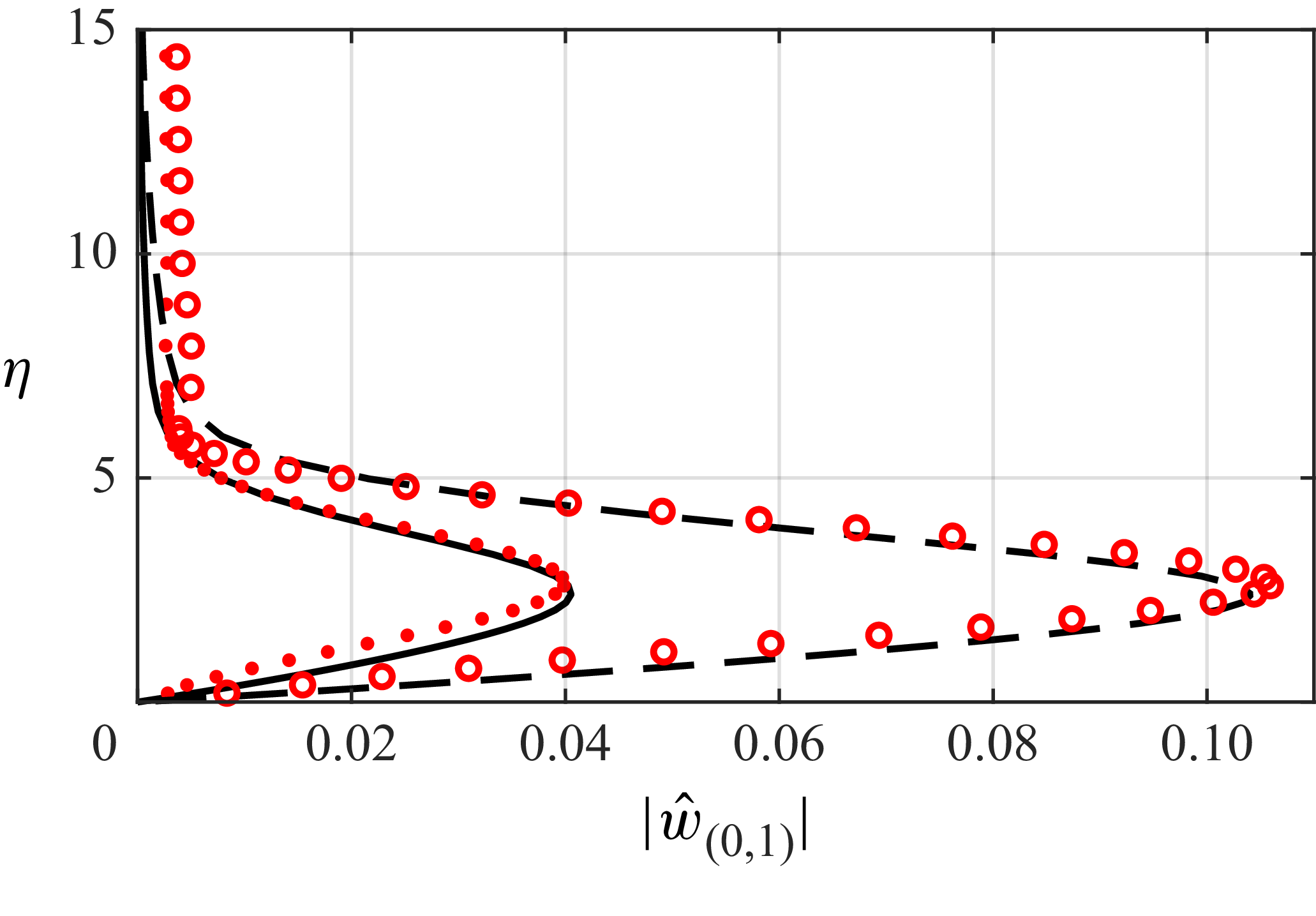
Figure 2. Spanwise perturbation velocity profile for mode

$(0,1)$
(

$\beta _1 = 0.1831$
) at the most upstream measurement plane in the experiments of Rius-Vidales et al. (Reference Rius-Vidales, Morais, Westerbeek, Casacuberta, Soyler and Kotsonis2025), corresponding to

$x = 527$
in the present work. HNS results (black lines) and experimental measurements (red markers) for the low-amplitude DRE case (solid line and small markers) and high-amplitude DRE case (dashed line and large markers).
At the solid wall

$(\eta =0)$
, all velocity-perturbation components are subject to homogeneous Dirichlet boundary conditions, enforcing no-slip and no-penetration. The perturbation pressure is solved implicitly and does not require a specific boundary condition. The outflow boundary is commonly associated with spurious reflections if left untreated as it interacts with incoming disturbances. This effect is particularly notorious in incompressible time-asymptotic formulations, see Kloker, Konzelmann & Fasel (Reference Kloker, Konzelmann and Fasel1993), Dobrinsky (Reference Dobrinsky2003) and Streett & Macaraeg (Reference Streett and Macaraeg1989) among others. To address this, an outflow buffer region in which downstream-travelling instabilities are artificially damped is implemented (see figure 1). The buffer region starts at 85 % of the total domain length

$L$
and extends to the outflow boundary. Herein, perturbations are gradually damped following a hyperbolic tangent distribution in

$x$
, see Westerbeek et al. (Reference Westerbeek, Hulshoff, Schuttelaars and Kotsonis2024) for details.
Homogeneous Dirichlet boundary conditions are imposed on the top boundary for all perturbation velocities to enforce the decay of perturbation modes in the inviscid free stream. An exception is made for the wall-normal velocity of the non-oscillatory MFD mode, which is left free to accommodate the spatial growth of the mean flow. A similar approach has been considered in NPSE computations (Herbert Reference Herbert1997). Additionally, the top boundary is placed sufficiently far from the wall to minimise potential artefacts stemming from the adaptation of the mean flow distortion in the vertical direction.
2.3.2. Discretisation
The system of spanwise-harmonic perturbation modes (2.4) is discretised in the wall-normal direction using a spectral collocation method with a Chebyshev polynomial basis. The differentiation matrix suite by Weideman & Reddy (Reference Weideman and Reddy2000) is used to provide the first and second-order differentiation matrices. Derivatives in the streamwise direction are approximated using a fourth-order central finite difference scheme for both the first- and second-order streamwise derivatives. For all investigated cases in this work, the domain was discretised using

$80$
Chebyshev collocation points in

$\eta$
that were clustered near the wall. In the chordwise direction,

$1500$
equispaced grid points are used. The results were subjected to a grid sensitivity study where both spatial axes were independently refined to ensure results were not significantly affected by the discretisation.
2.4. Energy-balance equations of the stationary spanwise-harmonic perturbations
The mechanisms of interaction between incoming CFI and the hump will be scrutinised by the use of energy-balance equations of the stationary spanwise-harmonic perturbation modes. These read as
(2.7)

\begin{equation} 0 = \mathcal{P}_{\beta _{n}} + \mathcal{T}_{\beta _{n}} + \mathcal{D}_{\beta _{n}} + \mathcal{W}_{\beta _{n}} + \mathcal{N}_{\beta _{n}}, \quad \textrm {with } \ n = 0,1, \ldots , N, \end{equation}
where

$n$
expresses the Fourier space of perturbations with spanwise wavenumber

$\beta _{n}$
and

$N$
is the number of spanwise modes considered.
Each term in (2.7) characterises a distinct mechanism of kinetic-energy transfer particular to perturbations of spanwise wavenumber

$\beta _{n}$
. Namely,
$\mathcal{P}_{\beta _{n}} = \mathcal{P}_{\beta _{n}}(x,y)$
expresses the exchange of kinetic energy between the unperturbed base flow and perturbations

$\beta _{n}$
,
$\mathcal{T}_{\beta _{n}} = \mathcal{T}_{\beta _{n}}(x,y)$
is the advection of kinetic energy of perturbations

$\beta _{n}$
by the base flow,
$\mathcal{D}_{\beta _{n}} = \mathcal{D}_{\beta _{n}}(x,y)$
characterises the viscous effects, and
$\mathcal{W}_{\beta _{n}} = \mathcal{W}_{\beta _{n}}(x,y)$
and
$\mathcal{N}_{\beta _{n}} = \mathcal{N}_{\beta _{n}}(x,y)$
respectively express the work of perturbation pressure and nonlinear interactions between harmonic modes and the mean flow distortion. By the stationary nature of perturbations, (2.7) expresses a balance; i.e. the corresponding physical mechanism remains in temporal equilibrium in the space of perturbations

$\beta _{n}$
. Inspection of the spatial behaviour of the terms of (2.7) provides insight into the evolution of corresponding physical mechanisms. Furthermore, their respective sign informs whether they act towards destabilising, i.e.

${\gt } 0$
, or stabilising, i.e.

${\lt } 0$
, perturbations

$\beta _{n}$
locally in space.
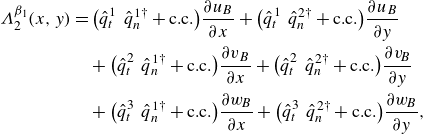
To aid in the analysis and interpretation of linear perturbation effects, the production term of (2.7) considering the fundamental perturbation,

$\beta _1$
, i.e.
(2.8)
\begin{equation} \mathcal{P}_{\beta _1} = – \frac {2 \pi }{\beta _1} \int _{S} \varLambda _{\beta _1} \, \textrm {d}x \,\textrm {d}y, \end{equation}
is decomposed as
(2.9)
\begin{align} \varLambda _{\beta _1}(x,y) = & \;\;\;\; \big ( \hat {u}^{\phantom {\dagger }}_{(0,1)} \hat {u}^{\dagger }_{(0,1)} + \textrm {c.c.} \big ) \frac {\partial u_{\! {B}}}{\partial x} + \big ( \hat {u}^{\phantom {\dagger }}_{(0,1)} \hat {v}^{\dagger }_{(0,1)} + \textrm {c.c.} \big ) \frac {\partial u_{\! {B}}}{\partial y} \nonumber\\ & + \big ( \hat {v}^{\phantom {\dagger }}_{(0,1)} \hat {u}^{\dagger }_{(0,1)} + \textrm {c.c.} \big ) \frac {\partial v_{\! {B}}}{\partial x} + \big ( \hat {v}^{\phantom {\dagger }}_{(0,1)} \hat {v}^{\dagger }_{(0,1)} + \textrm {c.c.} \big ) \frac {\partial v_{\! {B}}}{\partial y} \nonumber\\ & + \big ( \hat {w}^{\phantom {\dagger }}_{(0,1)} \hat {u}^{\dagger }_{(0,1)} + \textrm {c.c.} \big ) \frac {\partial w_{\! {B}}}{\partial x} + \big ( \hat {w}^{\phantom {\dagger }}_{(0,1)} \hat {v}^{\dagger }_{(0,1)} + \textrm {c.c.} \big ) \frac {\partial w_{\! {B}}}{\partial y}, \end{align}
where the dagger represents a complex conjugate, and

$u_B$
,

$v_B$
and

$w_B$
refer to the base flow velocities in the

$x$
-,

$y$
– and

$z$
-directions, respectively. The integration space

$S$
denotes a surface in the

$x$
–

$y$
plane that encompasses the hump in

$x$
and vertically extends from the wall to the free stream. Following the approach of Albensoeder, Kuhlmann & Rath (Reference Albensoeder, Kuhlmann and Rath2001), production is expressed into four contributions,
(2.10)
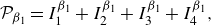
\begin{equation} \mathcal{P}_{\beta _1} = I^{\beta _1}_{1} + I^{\beta _1}_{2} + I^{\beta _1}_{3} + I^{\beta _1}_{4}, \end{equation}
each of which expresses a distinct mechanism relating the exchange of kinetic energy between the unperturbed base flow and fundamental perturbations (Lanzerstorfer & Kuhlmann Reference Lanzerstorfer and Kuhlmann2012; Loiseau, Robinet & Leriche Reference Loiseau, Robinet and Leriche2016; Picella et al. Reference Picella, Loiseau, Lusseyran, Robinet, Cherubini and Pastur2018). Equation (2.10) is obtained by introducing the perturbation decomposition
(2.11)
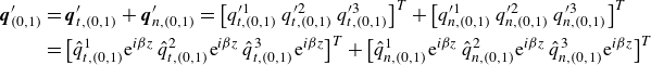
\begin{align} \boldsymbol{q}^{\prime }_{(0,1)} & = \boldsymbol{q}^{\prime }_{t,(0,1)} + \boldsymbol{q}^{\prime }_{n,(0,1)} = \big[q^{\prime 1}_{t,(0,1)} \; q^{\prime 2}_{t,(0,1)} \; q^{\prime 3}_{t,(0,1)}\big]^{T} + \big[q^{\prime 1}_{n,(0,1)} \; q^{\prime 2}_{n,(0,1)} \; q^{\prime 3}_{n,(0,1)}\big]^{T} \nonumber\\ & = \big[\hat {q}^{1}_{t,(0,1)} \textrm {e}^{ {i} \beta z} \; \hat {q}^{2}_{t,(0,1)}\textrm {e}^{ {i} \beta z}\; \hat {q}^{3}_{t,(0,1)}\textrm {e}^{ {i} \beta z}\big]^{T} + \big[\hat {q}^{1}_{n,(0,1)} \textrm {e}^{ {i} \beta z} \; \hat {q}^{2}_{n,(0,1)}\textrm {e}^{{i} \beta z}\; \hat {q}^{3}_{n,(0,1)}\textrm {e}^{ {i} \beta z}\big]^{T} \end{align}
into the original form of production, where the superscripts

$1$
,

$2$
and

$3$
here denote vector components in the

$x$
-,

$y$
– and

$z$
-directions, respectively. In (2.11), the vector field

$\boldsymbol {q}^{\prime }_{t}$
characterises the perturbation that is locally tangent to the base flow streamlines; i.e. pointing in the local direction of the (base) flow. The complementary vector field

$\boldsymbol {q}^{\prime }_{n}$
characterises the perturbation that is locally normal to the base flow streamlines; i.e. which acts in the cross-stream direction. It must be noted that both

$\boldsymbol {q}^{\prime }_{t}$
and

$\boldsymbol {q}^{\prime }_{n}$
are stationary spanwise-periodic perturbation fields. The reader is referred to Casacuberta et al. (Reference Casacuberta, Hickel, Westerbeek and Kotsonis2022) and Casacuberta, Hickel & Kotsonis (Reference Casacuberta, Hickel and Kotsonis2024) for explicit analytic expressions of

$\boldsymbol {q}^{\prime }_{t}$
and

$\boldsymbol {q}^{\prime }_{n}$
, as well as details on their mathematical formulation.
The term

$I^{\beta _1}_2$
of (2.10) will be shown to add the main contribution to production

$\mathcal{P}_{\beta _1}$
. It reads as
(2.12)
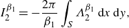
\begin{equation} I^{\beta _1}_{2} = – \frac {2 \pi }{\beta _1} \int _{S} \varLambda ^{\beta _1}_{2} \, \textrm {d}x \,\textrm {d}y, \end{equation}
with
(2.13)
\begin{align} \varLambda ^{\beta _1}_{2}(x,y) & = \big ( \hat {q}^{1\phantom {\dagger }}_{t} \hat {q}^{1 \dagger }_{n} + \textrm {c.c.} \big ) \frac {\partial u_{{B}}}{\partial x} + \big ( \hat {q}^{1\phantom {\dagger }}_{t} \hat {q}^{2 \dagger }_{n} + \textrm {c.c.} \big ) \frac {\partial u_{{B}}}{\partial y} \nonumber\\ & \quad + \big ( \hat {q}^{2\phantom {\dagger }}_{t} \hat {q}^{1\dagger }_{n} + \textrm {c.c.} \big ) \frac {\partial v_{{B}}}{\partial x} + \big ( \hat {q}^{2\phantom {\dagger }}_{t} \hat {q}^{2\dagger }_{n} + \textrm {c.c.} \big ) \frac {\partial v_{\! {B}}}{\partial y} \nonumber\\ & \quad + \big ( \hat {q}^{3\phantom {\dagger }}_{t} \hat {q}^{1\dagger }_{n} + \textrm {c.c.} \big ) \frac {\partial w_{\! {B}}}{\partial x} + \big ( \hat {q}^{3\phantom {\dagger }}_{t} \hat {q}^{2\dagger }_{n} + \textrm {c.c.} \big ) \frac {\partial w_{\! {B}}}{\partial y}, \end{align}
where the subindex

$(0,1)$
is removed for conciseness. The

$I^{\beta _1}_2$
characterises the well-known lift-up effect (Ellingsen & Palm Reference Ellingsen and Palm1975; Landahl Reference Landahl1975), i.e. the exchange of kinetic energy between the unperturbed base flow and streamwise-tangent perturbations,

$\boldsymbol {q}^{\prime }_{t}$
, by the action of cross-stream perturbations,

$\boldsymbol {q}^{\prime }_{n}$
. A treatment analogous to (2.12) and (2.13) may be performed for the remaining terms of decomposition (2.10), namely

$I^{\beta _1}_{1}$
,

$I^{\beta _1}_{3}$
and

$I^{\beta _1}_{4}$
, see Casacuberta et al. (Reference Casacuberta, Westerbeek, Franco, Groot, Hickel, Hein and Kotsonis2025).
2.5. Advection perturbation equations
A so-called perturbation advection framework complements the analysis of the energy-balance equations presented already. As will be shown in the following discussion, the presence of the smooth surface hump significantly distorts the organisation of both the base flow and the stationary perturbation field. Towards isolating this effect, a framework is introduced to simulate base-flow advection of incoming perturbations. Isolating the perturbation convection term from (2.4a
), i.e. neglecting production, pressure effects, nonlinear interactions and viscous effects for a stationary flow, yields
(2.14)
\begin{equation} (\boldsymbol{Q} \boldsymbol{\cdot } \boldsymbol{\nabla }) \boldsymbol{q’} = 0, \end{equation}
where the perturbation ansatz is identical to that of the HNS framework (see (2.5)). Physically, the solution of (2.14) governs the advection of an incoming perturbation profile according to the three-dimensional streamlines of the base flow, akin to a scalar transport process. The perturbation advection framework is numerically implemented as an adaptation of the HNS framework and employs the same discretisation and boundary conditions as a result.
3. Topology of the base flow
With the hump present, the organisation of the unperturbed steady base flow is altered significantly. This section describes the evolution of the base flow in the vicinity of the hump and compares it with the reference case (i.e. no hump present). The focus lies on the development of base flow quantities in the vicinity of the hump that are known to be important to the flow stability.
3.1. Effect of the hump on the base flow boundary layer
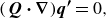
The spatial evolution of the chordwise pressure gradient,

$\partial P / \partial x$
, and key boundary layer parameters are illustrated in figure 3.
The boundary layer thicknesses are measured from the local (deformed) wall in the direction normal to the reference clean wing surface and presented against the

$\eta$
coordinate. The hump strongly affects all boundary layer quantities at the hump location and in its proximity. Distortions can be seen in the chordwise region from

$x =450$
(all spatial coordinates are non-dimensionalised with

$l_{\textit{ref}}$
, see table 1) onward, while the boundary layer recovers to the reference conditions around

$x\approx 820$
. The hump incurs a notable distortion as well on the pressure gradient field, initially decelerating the flow and thickening the boundary layer. As the flow traverses the hump, it experiences successive acceleration and deceleration events.
The skin friction coefficient remains positive throughout the streamwise extent of the hump, thus signifying the absence of laminar separation and reverse flow in the chordwise direction. Previous studies on the effect of surface features on incoming CFI linked the formation of a local region of reverse flow with the rapid spatial growth of CFI (Hosseinverdi & Fasel Reference Hosseinverdi and Fasel2016; Xu et al. Reference Xu, Lombard and Sherwin2017; Westerbeek et al. Reference Westerbeek, Franco Sumariva, Michelis, Hein and Kotsonis2023). The absence of reverse flow around the hump in the present work ensures that the alteration of the behaviour of CFI at the hump is not explicitely driven by such effects.
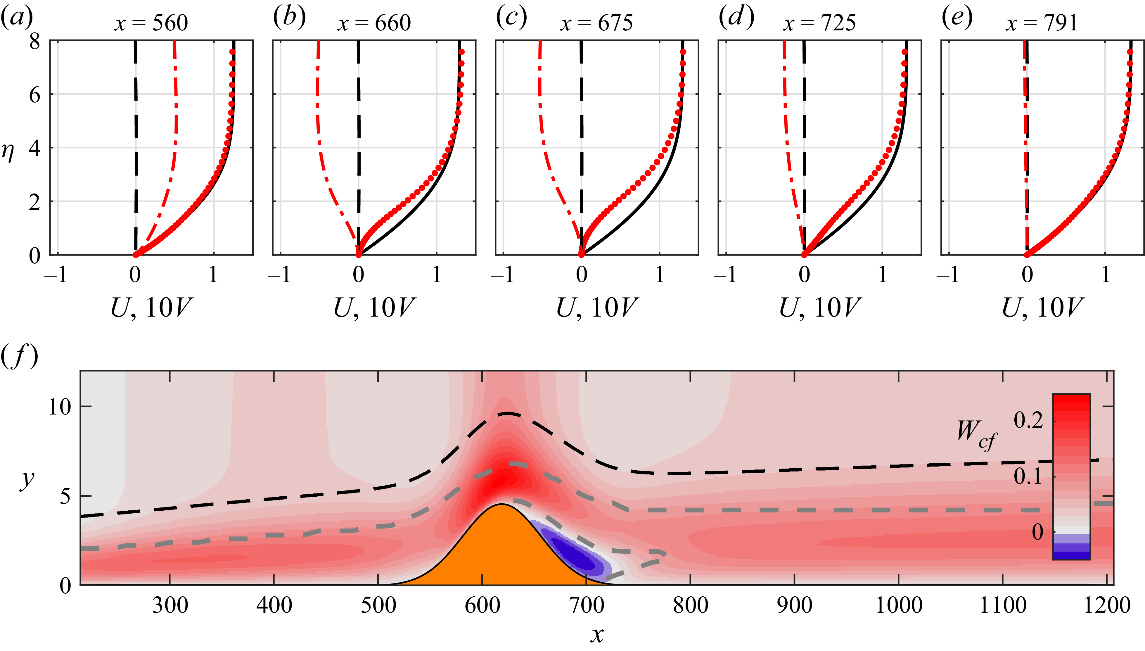
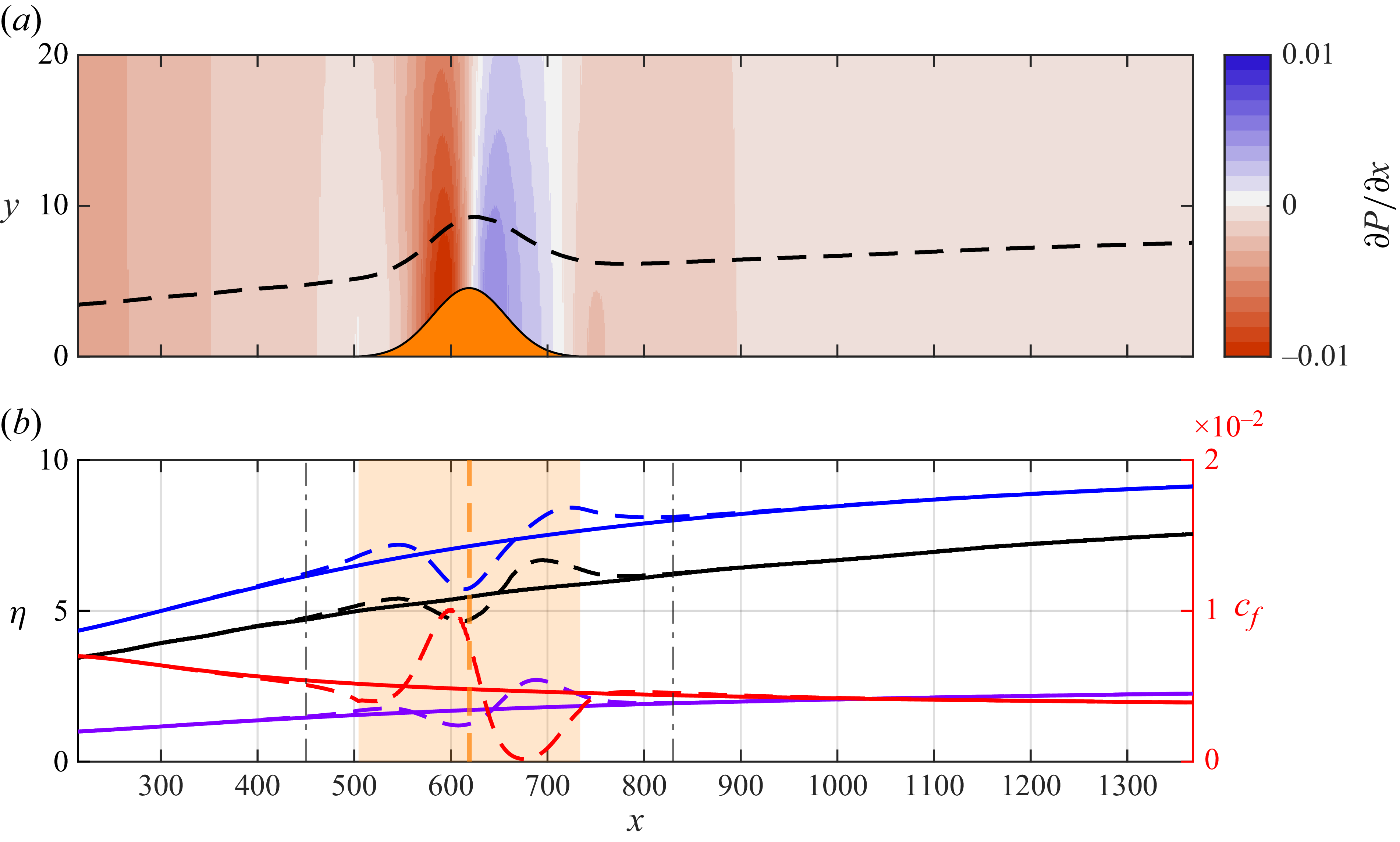
Figure 4. (a–e) Base flow components of chordwise velocity (

$U$
) (red dotted and black solid lines) and wall-normal velocity (

$V \times 10$
) (red dash-dotted and black dashed lines) in the hump (red) and reference (black) cases. (f) Spatial evolution of the cross-flow velocity in the hump case. Black dashed line indicates the

$\delta _{99}.$
Grey dashed lines indicate loci of inflection points. The hump is indicated in orange.
The effect of the hump on the base flow velocity profiles is quantitatively illustrated in figure 4. The hump alters the evolution of the wall-normal velocity of the base flow, effectively creating a transversal motion of successive upwash and downwash events in

$x$
. This effect extends further than the viscous region (i.e.

$\eta \gt \delta _{99}$
). The chordwise velocity experiences a rapid deceleration in

$x$
as a result of the hump-induced pressure gradient. This is particularly accentuated in the near-wall region (i.e.

$\eta \lt 4$
). However, in contrast to the wall-normal velocity, this effect largely diminishes outside the boundary layer.
3.2. Cross-flow reversal
Cross-flow reversal, i.e. the inversion of the direction of the cross-flow velocity component, is captured in the downstream vicinity of the hump apex in figure 4( f). The cross-flow component is defined as the velocity component orthogonal to the external inviscid streamline. Granted its inflectional shape, it is widely acknowledged to be the driving source of the cross-flow instability (Saric et al. Reference Saric, Reed and White2003). The local and rapid chordwise change of pressure gradients by the hump leads to cross-flow reversal. Within the scope of incoming CFI interacting with forward-facing step flow, Tufts et al. (Reference Tufts, Reed, Crawford, Duncan and Saric2017) ascribe cross-flow reversal to the effect of local adverse pressure gradients. Moreover, Eppink (Reference Eppink2020) states that the modification of the cross-flow velocity in the vicinity of a forward-facing step influences the rotation direction of the cross-flow instability at the step. Despite the shallow hump shape, cross-flow reversal arises prominently in the presently investigated flow (figure 4
f).
In juxtaposition to geometry-induced modification of pressure gradients, Wassermann & Kloker (Reference Wassermann and Kloker2005) investigated the effect of external (i.e. inviscid) pressure gradient change-over on the development of stationary CFI. Wassermann & Kloker (Reference Wassermann and Kloker2005) report that the pressure gradient change-over induces reversal of the cross-flow component in the boundary layer. The results of a linear local stability analysis demonstrated that the adverse pressure gradient (APG) and subsequent cross-flow reversal act towards stabilising the incoming CFI in a modal sense. The authors concluded that ‘the reversed basic cross-flow close to the wall leads to a redistribution of spanwise shear in the mean flow distorted by the steady cross-flow vortices coming from upstream’. This may be partially reconciled with the observed stabilisation of CFI by the hump in the experiments of Rius-Vidales et al. (Reference Rius-Vidales, Morais, Westerbeek, Casacuberta, Soyler and Kotsonis2025), but raises questions on how the stabilisation effect is dependent on the amplitude of incoming instabilities, as quantitatively characterised in this present work. Furthermore, Wassermann & Kloker (Reference Wassermann and Kloker2005) studied the response of the boundary layer to the change-over from favourable pressure gradient (FPG) to APG without reverting to FPG, which is the flow environment in the hump case.
In the present scenario, the cross-flow component reverts direction almost immediately downstream of the hump apex. The region of cross-flow reversal extends from

$x = 640$
to

$x =725$
. The peak of reverse cross-flow velocity reaches a maximum in

$x$
of approximately

$ -0.05\bar {U}_{\textit{ref}}$
. However, just upstream of the hump apex, the cross-flow component is significantly strengthened, i.e. in the classic direction, in comparison to reference conditions, due to the enhanced favourable pressure gradient by the hump. Cross-flow reversal is also localised in the wall-normal direction, i.e. it does not extend far into the upper boundary layer. In a fashion similar to the work of Hosseinverdi & Fasel (Reference Hosseinverdi and Fasel2016), cross-flow reversal here extends from the wall to approximately

$\eta = 2$
. This can be attributed to the lower local spanwise momentum in this region of the boundary layer. Sufficiently downstream of the hump, the base flow relaxes to reference conditions; from

$x=730$
, the cross-flow component returns to the classic positive direction.
4. Evolution of the perturbation field
To analyse the response of the perturbation field to the presence of the hump, linear and nonlinear formulations of the HNS framework are used. In both cases, the perturbation evolution is initiated by the amplification in

$x$
of the fundamental CFI mode. As described in § 2, a stationary (i.e. zero temporal frequency) cross-flow eigenmode with fundamental spanwise wavelength,

$\beta _1 = 0.1831$
, is prescribed at the inflow. This is computed as the solution to the local Orr–Sommerfeld eigenvalue problem. Linear HNS simulations account solely for the growth of the fundamental cross-flow mode. In contrast, the effect of finite-amplitude cross-flow perturbations on the interaction mechanism with the hump is assessed using the fully nonlinear HNS framework.
4.1. Effect of the hump on linear perturbation
The spatial amplification of the fundamental CFI is quantified in figure 5. Instability growth is largely unaffected by the presence of the hump up to its leading edge (i.e.

$x\lt 500$
). In contrast, the impact of the hump on the CFI development manifests both locally in the vicinity of the hump as well as further downstream of it.
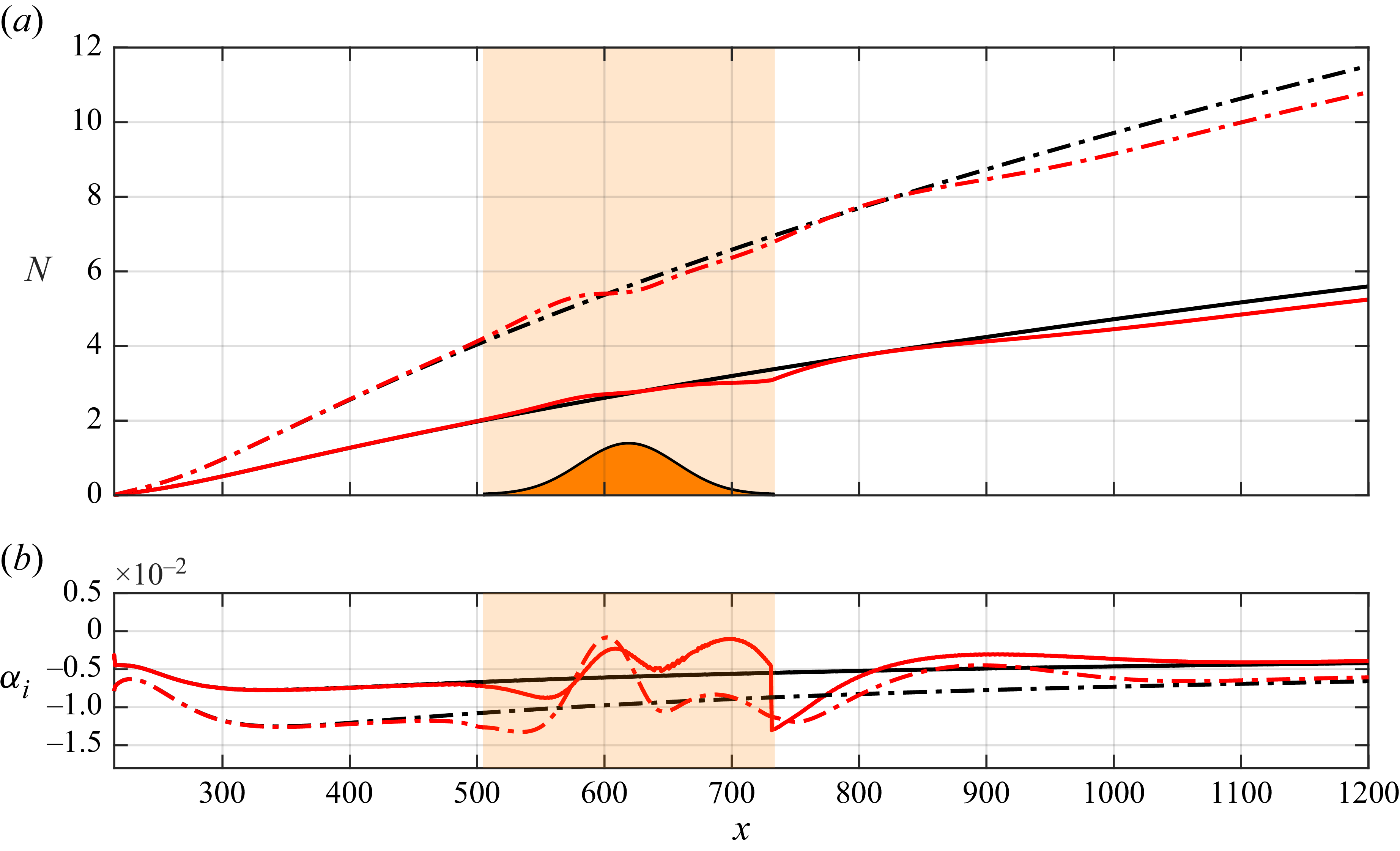
Figure 5. Spatial evolution of the fundamental CFI mode (

$\beta _1 = 0.1831$
) in the hump (red) and reference (black) cases quantified as: (a) amplification factor,

$N$
, based on the peak of chordwise velocity perturbation (solid lines) and total perturbation kinetic energy

$E_k$
(dash-dotted lines); and (b) spatial growth rate. Growth metrics are based on the peak of chordwise velocity perturbation (solid and dashed lines) and on total perturbation kinetic energy (dash-dotted lines). Orange shaded region indicates the hump’s spatial extent.
The perturbation amplification factor,

$N$
, is depicted in figure 5(a). The N-factor is calculated locally as
(4.1)
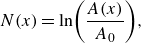
\begin{equation} N(x) = \text{ln}\!\left (\frac {A(x)}{A_0}\right )\!, \end{equation}
with the amplitude measure

$A$
based on either the maximum of the chordwise velocity perturbation or the wall-normal integral of perturbation kinetic energy (§ 2). The reference amplitude

$A_0=A(x_0)$
is taken at the domain inflow (

$x_0 = 214l_{\textit{ref}})$
. Growth rates based on these two quantities, see equation (2.6) are additionally illustrated in figure 5(c). The evolution of growth rates is qualitatively similar. Specifically, the effect of the hump on the incoming instability can be decomposed into three distinct regions. The first region spans approximately the upstream half of the hump (i.e.
$500 \leqslant x \leqslant 580$
). In this range, the CFI is destabilised, when compared with reference conditions. This trend correlates with the spatial deceleration of chordwise base flow velocity and concurrent increase in the cross-flow component, as evident in figure 4. Conversely, the second region (i.e.
$580 \leqslant x \leqslant 800$
) coincides partly with the cross-flow reversal seen in the base flow. In this region, the CFI stabilises in the vicinity of the hump’s apex and shortly downstream of it. In contrast, upstream of the hump’s trailing edge (

$x\approx 720$
), the growth rates become again lower than reference values.
Finally, a third region of evident growth rate modification due to the hump is identified (i.e.

$800 \leqslant x \leqslant 1100$
). Within this region, the hump appears to have a significant and persistent effect on the perturbation growth rate as downstream as

$x\approx 1100$
, in a range of approximately two hump lengths downstream of the hump’s apex. This is in stark contrast to the effect of the hump on the base flow. The latter is effectively recovered to the reference case from

$x\approx 820$
onward, as shown in figures 3 and 4. In combination, the incoming CFI experiences successive events of stabilisation and destabilisation as it traverses over the hump. However, in an integral manner, the instability exits the hump’s region of influence and recovers to the reference growth rate at

$x\approx 1100$
with almost 60 % of the amplitude of the reference case (

$\Delta N\approx -0.5$
based on

$|u’|$
), further reconciling with the experimental observations of transition delay by Rius-Vidales et al. (Reference Rius-Vidales, Morais, Westerbeek, Casacuberta, Soyler and Kotsonis2025).
To gain insight into the effect of the hump on the perturbation evolution locally at the hump, as well as downstream of it, the amplitude shape profile (see (2.5)) is inspected in figure 6. For the purpose of this analysis, only the chordwise (

$\hat {u}$
) and wall-normal (

$\hat {v}$
) amplitude functions are considered. The spanwise velocity component

$\hat {w}$
is not shown here as it largely resembles

$\hat {u}$
. As the incoming CFI ascends the hump, the wall-normal perturbation velocity is amplified, which is then largely compensated during the descent downstream of the hump apex. In contrast, the chordwise component (

$\hat {u}$
) demonstrates a more complex response. The shape profile

$\hat {u}$
shows a near-wall deficit compared with the reference case upstream of the hump apex. This is accompanied by an overall broadening of the shape profile and displacement of its local maximum further away from the wall. In this regard, the perturbation shape follows the behaviour of the base flow closely (figure 4). This is further reconciled by a consistent and evident correlation of the wall-normal location of maximum

$|\hat {u}|$
with the location of inflection points in the cross-flow velocity profiles of the base flow (identified by blue dashed lines in figure 6 and visualised in figure 4
f).
The resultant modifications in perturbation shape are also linked to changes in amplitude. In the vicinity of the hump apex and immediately downstream of it, the perturbation experiences a rapid spatial amplification accompanied by a displacement of the peak perturbation velocity towards the wall. Within a short chordwise range (
$718\lt x\lt 739$
), the

$\hat {u}$
profile features two local maxima. For comparison, the base flow cross-flow component experiences reversal and, as a consequence, features two inflection points in the chordwise region
$719\lt x\lt 740$
.
The concurrent presence of two maxima is responsible for a pronounced discontinuity in the growth rate derived from the maximum of chordwise perturbation velocity at

$x\approx 740$
, as shown in figure 5(c). At this location, the maximum perturbation velocity switches between the two local peaks, thus the evolution of the growth rate in

$x$
is not continuous. Naturally, this does not manifest in the energy-based growth rate due to its integral evaluation. A double-peak topology of the

$u$
-perturbation shape has been reported in previous studies involving CFI interacting with a hump (Westerbeek et al. Reference Westerbeek, Franco Sumariva, Michelis, Hein and Kotsonis2023), as well as a forward-facing step (Casacuberta et al. Reference Casacuberta, Hickel and Kotsonis2021, Reference Casacuberta, Hickel, Westerbeek and Kotsonis2022). Casacuberta et al. (Reference Casacuberta, Hickel and Kotsonis2021) argue that the near-wall peak is the manifestation of an additional perturbation structure (namely, perturbation streaks) that forms locally at the upper step corner and co-exist with the CFI developing above and farther from the wall.
4.2. Local and non-local linear stability analysis
Due to the convective nature of the CFI, the perturbation development at any chordwise location is expected to be strongly dependent on its spatial history. The global nature of the HNS formulation, which is based on the full NS equations, can capture this dependency. In contrast, the unique quality of locality of the Orr–Sommerfeld (OS) operator renders it insensitive to the history of the perturbation and the chordwise variation of the base flow. Thus, these effects can be segregated by comparing the solutions of local stability analysis for the fundamental mode with the corresponding solution of the linear HNS equations. Towards this goal, the alteration of the perturbation shape at the hump may be ascribed to the changes in the local eigensolution and the rise of new unstable modes as a consequence of the altered base flow.
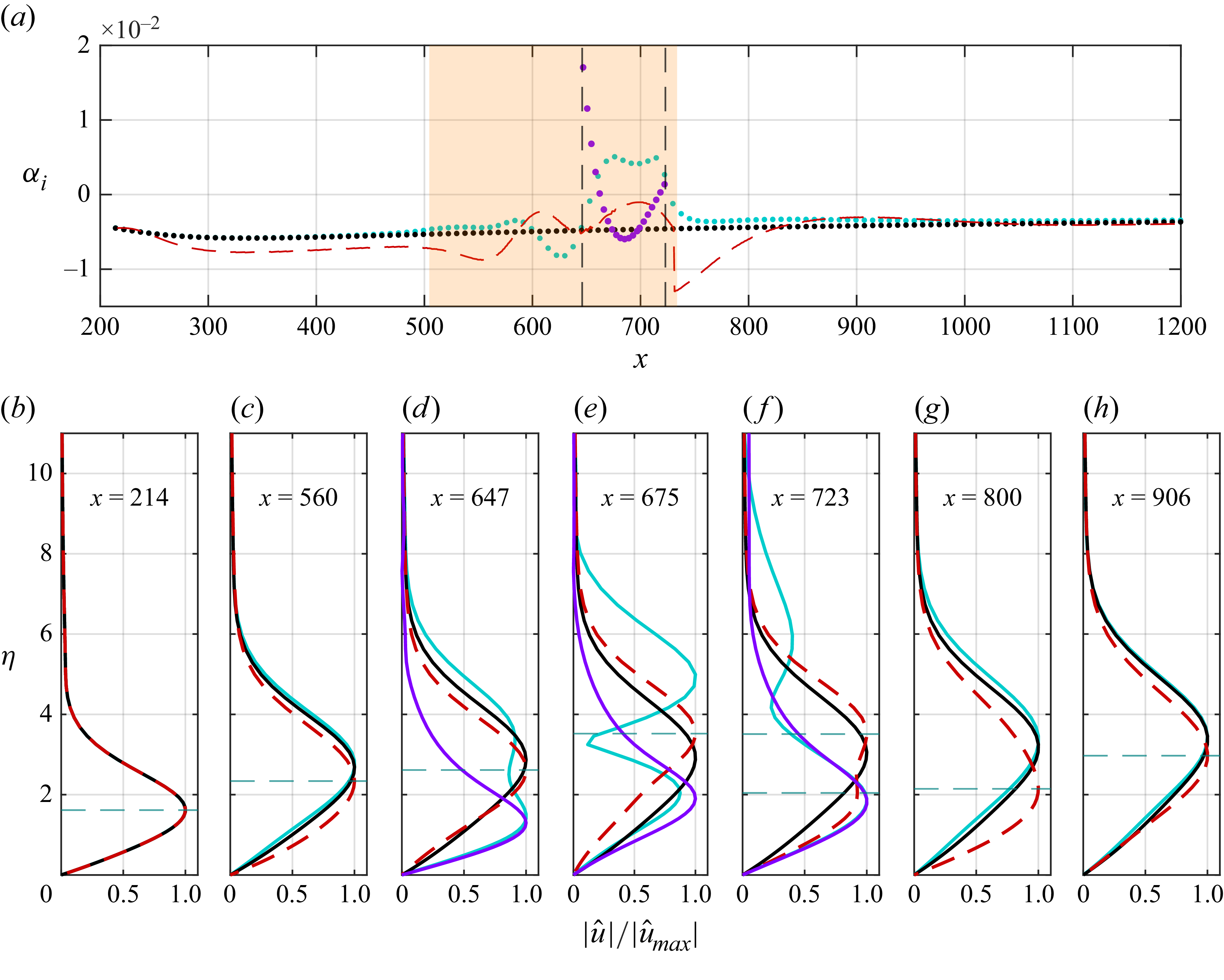
Figure 7. (a) Orr–Sommerfeld spatial growth rate

$\alpha _i$
for

$\beta _1 = 0.1831$
in the hump case corresponding to the original CFI mode tracked from the inflow (cyan markers) and a novel near-wall mode in the CF reversal region (purple markers). Reference case is shown in black markers. Corresponding HNS solution in the hump case is shown for comparison (red dashed line). Orange shaded region denotes the spatial extent of the hump. Vertical dashed lines indicate the region of cross-flow reversal in the base flow. (b–h) Local eigenfunction shape of chordwise velocity at selected chordwise stations in the hump case (cyan and purple solid lines, corresponding to the original and new near-wall CFI modes, respectively) and reference case (black solid line). Corresponding HNS solution in the hump case is shown for comparison (red dashed line). Horizontal dashed lines indicate the location of inflection points in the base flow cross-flow profile.
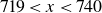
The Orr–Sommerfeld analysis is carried out in the range
$x \in [214, 1200]$
at 1500 equally distributed stations for the hump and reference cases. Selected eigensolutions of the local OS eigenspectrum are portrayed in figure 7. Based on the spatial stability formulation of the problem, results are interpreted in terms of the complex eigenvalue

$\alpha =\alpha _r + \textrm {i}\alpha _i$
, for which the real component corresponds to the chordwise wavenumber of the instability mode (not shown here), while the imaginary component expresses the chordwise growth rate. The spatial growth rate computed from the peak chordwise perturbation velocity obtained from HNS, see equation (2.6) is shown for reference. It must be stressed that the HNS solution considers a series of terms in the Navier–Stokes equations that are neglected in the OS formulation, such as the chordwise flow derivatives. As such, even for the reference case, slight deviations in the growth rate predicted by the two approaches are measured. This is particularly evident at upstream locations in the domain (

$x\lt 500$
), where the boundary layer is strongly accelerating in

$x$
and non-parallel effects are non-negligible in the HNS solution (figure 7).
The growth rates obtained as solutions to the OS and HNS equations are significantly affected by the presence of the hump. The fundamental local CFI mode (cyan markers in figure 7
a) starts to deviate from the reference case at approximately

$x = 500$
. Within the range occupied by the hump (
$500\lt x\lt 720$
), the differences between OS and HNS solutions are also evident in the shape of corresponding eigensolutions. The shape function of the OS eigenmode develops a double-peak structure rapidly in

$x$
(see figure 7
d–f) and returns to the single-peaked structure immediately downstream of the hump. Particularly evident in a short region downstream of the hump’s apex (
$621\lt x\lt 740$
) is the secondary peak in the near-wall region (

$\eta \approx 2$
). This range shows a strong correlation to the region of cross-flow reversal (indicated by the vertical dashed lines in figure 7) and is accompanied by rapid spatial stabilisation in

$x$
, evident by the positive OS growth rate. In contrast, the HNS solution experiences a largely milder spatial evolution, with a double-peak structure only briefly manifesting at the downstream end of the hump (

$x\approx 723$
). Similarly, the growth rate calculated by HNS experiences a shift to less unstable values, albeit remaining negative. The inability of the OS solution to reconcile with the corresponding HNS growth rate in the range
$500\lt x\lt 1100$
is strongly suggestive of growth mechanisms active in this region which cannot be described on the basis of local purely parallel eigensolutions. This will be discussed in §§ 4.3 and 4.4.
Interestingly, the modified boundary layer due to the hump supports a new instability eigenmode. This appears in the OS eigenspectrum downstream of the hump apex at

$x=647$
and is located in the unstable half-plane in the short chordwise extent between

$x\approx 660$
and

$x\approx 710$
(see purple markers in figure 7
a). The OS operator admits this mode as a valid, albeit only briefly unstable, solution to the local boundary layer stability. This mode is not directly evident in the HNS solution, but similarities in the shape profile are observed. The presence of an OS eigensolution, additional to the incoming CFI and qualitatively resembling the behaviour of the one identified here, was described by Krochak et al. (Reference Krochak, Casacuberta, Hickel and Kotsonis2022) in backward-facing step flow and associated with a new inflection point appearing in addition to the classical inflection of crossflow velocity profiles shortly downstream of the step apex.
To further elucidate the character of the modified CFI in relation to the novel near-wall mode induced by the hump, their mode shapes are examined in the

$\eta {-}z$
plane, normalised by their respective maximum. Specifically, the chordwise velocity component of the local stability solution is expanded in the spanwise direction through the application of the OS harmonic ansatz and displayed in figure 8(a–g) for the incoming CFI mode (cyan lines in figure 7
b–h). For reference, the HNS solution is shown in figure 8(h–n). The local CFI mode predicted by the OS solution experiences significant topological changes due to the hump. At

$x=647$
, a localised deformation in the profile occurs as the structure tilts to the positive

$z$
-axis near the wall. This is strongly reminiscent of the observations of Wassermann & Kloker (Reference Wassermann and Kloker2005) who studied the effect of a favourable to adverse pressure gradient (FPG to APG) change-over on the evolution of stationary CFI. The evolution of the mode topology downstream of the hump’s apex is noteworthy. The mode is continuously stretched in the

$z$
-direction and evolves from a classical cross-flow instability shape to a distinct out-of-phase double-peak structure (figure 8
d). Concurrently, in the region where the double peak forms and near-wall phase inversion is mostly active (
$650\lt x\lt 720$
), the mode is predicted to be linearly stable by the OS operator, i.e.

$\alpha _i\gt 0$
(figure 7). In the same region, the HNS solution is found to be stabilised, in comparison with the reference case.
Figure 8. Spanwise harmonic reconstruction of (a–g) local OS and (h–n) HNS solutions of the incoming CFI mode normalised by

$u’_{{max}}$
. The chordwise perturbation velocity is illustrated, considering contour levels from

$-1$
(blue) to

$1$
(red) at selected chordwise stations.
The origin of deformation of the CFI into a double-peak structure is further explored here through a simple heuristic experiment, where a pre-existing perturbation system is exposed to pure scalar transport by the base flow. This is facilitated directly within the HNS framework, by disabling all terms in the HNS equations except the advection term, as outlined in § 2.5. The effect of scalar transport on a pre-computed perturbation obtained as a solution to the Orr–Sommerfeld eigenvalue problem and introduced at the

$x$
-location of the hump apex is shown in figure 9 for both hump and reference cases. The perturbation system that advects over the hump is found to be prominently tilted in the

$y{-}z$
plane, as opposed to the reference case, due to the cross-flow reversal. Although many other important flow mechanisms are neglected, the resulting shape closely resembles the double-peaked shape observed in the full HNS simulation and the OS analysis (figure 8). This further confirms a key element in the overall mechanism of stability manipulation by the hump, namely the spanwise transport varying with the distance from the wall and the resulting distortion of incoming CFI.
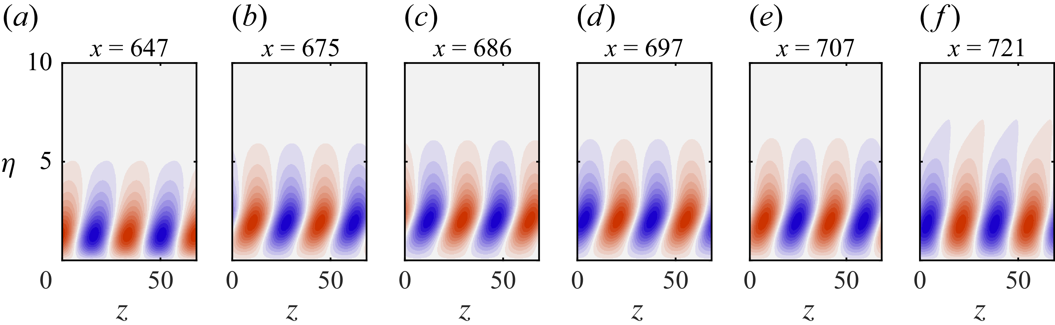
Figure 10. Spanwise harmonic reconstruction of the local OS (secondary) unstable near-wall mode normalised by

$u’_{{max}}$
. The chordwise perturbation velocity is illustrated, considering contour levels from

$-1$
(blue) to

$1$
(red) at selected chordwise stations.
Finally, the origin and influence of the novel near-wall unstable eigenmode shown in figure 10 are briefly discussed. This perturbation resembles a classic cross-flow instability in a structural sense. However, in contrast to the incoming CFI shown in figure 8, the mode shape in the

$\eta {-}z$
plane of the new near-wall mode is tilted anti-clockwise. This can also be traced back to the topology of the local base flow, as this new eigenmode destabilises purely within the region of cross-flow reversal (figure 4). This reconciles with the results of Eppink (Reference Eppink2020) and Krochak et al. (Reference Krochak, Casacuberta, Hickel and Kotsonis2022) for CFI-dominated flows over backward-facing steps, where the presence of step-induced inflectional profiles embedded in a region of cross-flow reversal was reported to give rise to new stationary instability modes near the wall. The newly identified OS eigenmode in the present work rapidly stabilises once it exits the cross-flow reversal region. As such, in conditions of pure linear instability growth, the near-wall mode is unlikely to reach a significant amplitude to be observable as a separate mode co-existing with the original incoming CFI. Therefore, its role in linear or low instability amplitude scenarios is likely to be minor. However, as will be shown in the following sections, the role of such near-wall modes can be elevated in importance in environments of high-amplitude and nonlinear instability development.
4.3. Nonlinear effects in CFI-hump interactions
The finite amplitude of incoming CFI interacting with a hump was found to significantly influence the transition location in the experiments of Rius-Vidales et al. (Reference Rius-Vidales, Morais, Westerbeek, Casacuberta, Soyler and Kotsonis2025), thus suggesting a key role played by the nonlinear perturbation effects. In the present section, these effects are investigated numerically by varying the inflow amplitude of the pre-imposed fundamental CFI mode (§ 2.3) in a fully nonlinear HNS framework. All other parameters, such as base flow, geometry and wave specifications, are kept identical to the linear analysis described in §§ 4.1 and 4.2. The evolution of the fundamental CFI (i.e.

$\beta = \beta _1$
), its four high-order harmonics (i.e.

$\beta = \beta _n, n = 2$
–

$5$
) and the mean flow distortion (MFD, i.e.

$\beta = 0$
) are considered here. The initial amplitude of the fundamental perturbation is varied from

$A_0 = 1.1 \times 10^{-3}$
to

$1.4\times 10^{-2}$
, while all other harmonics and the MFD are initiated as null at the domain inflow. The MFD and higher harmonics arise naturally in

$x$
through nonlinear interactions.
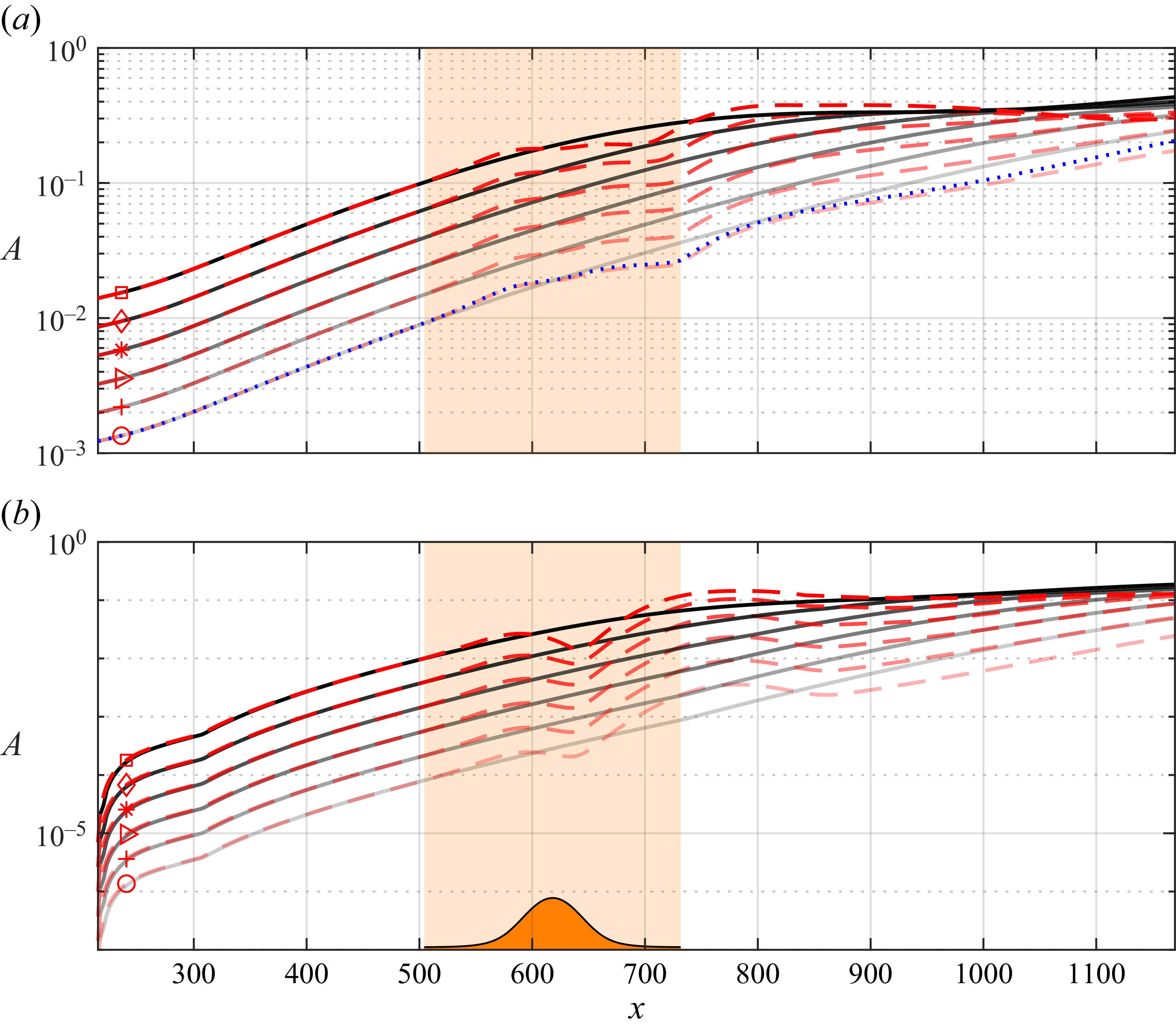
Figure 11. Amplitude of (a) fundamental mode

$\beta = \beta _{1}$
and (b) first harmonic mode

$\beta = \beta _{2}$
in the hump (red) and reference cases (black) for inflow amplitudes

$A_0= [0.12, 0.20, 0.32, 0.53, 0.86, 1.40] \times 10^{-2}$
marked respectively by the circle, plus, triangle, asterisk, diamond and square markers at the inflow. Increasing opacity of lines indicates an increase in amplitude. The hump and its chordwise extent are indicated in orange. Purely linear amplitude evolution, obtained by linearised HNS, is indicated by dotted blue line.
The chordwise evolution of the amplitude of the fundamental mode

$\beta = \beta _{1}$
and the harmonic

$\beta = \beta _{2}$
are illustrated in figure 11. For the lowest initial amplitude considered in this work, the perturbation evolution is linearly dominated in the entire domain. Consequently, nonlinear mechanisms increasingly dominate the behaviour as the inflow amplitude of the fundamental perturbation is increased. Significant qualitative differences can also be observed between the amplitude evolution of the

$\beta = \beta _{1}$
and

$\beta = \beta _{2}$
modes as a function of inflow amplitude. However, higher harmonics follow a trend closely resembling the

$\beta = \beta _{2}$
mode. Hence, the behaviour of modes with

$\beta \gt \beta _{2}$
is here disregarded in the discussion of results. For low initial amplitudes, the fundamental mode is generally stabilised and exits the simulation domain at a significantly lower amplitude than in the corresponding reference case (figure 11
a). This is also observed in the results of the purely linear simulation. The amplitude reduction occurs effectively at all chordwise positions downstream of the hump’s apex. In contrast, as the inflow amplitude increases, an increasingly strong destabilisation is observed at the downstream end of the hump (i.e.

$x \approx$
720). For initial mode amplitudes greater than
$A_0 = 5.3 \times 10^{-3}$
, the CFI downstream of the hump attains amplitudes higher than the associated reference case despite then decaying to a lower amplitude further downstream.
Linear growth of CFI is followed by subsequent stages of nonlinear growth and saturation-like behaviour, i.e. quasi-saturation, as reported in numerical (Wassermann & Kloker Reference Wassermann and Kloker2002; Casacuberta et al. Reference Casacuberta, Hickel, Westerbeek and Kotsonis2022) and experimental (Arnal Reference Arnal1994; Reibert et al. Reference Reibert, Saric, Carrillo and Chapman1996) work as well as nonlinear stability analysis (Haynes & Reed Reference Haynes and Reed2000). This originates from nonlinear energy exchange between harmonic modes and particularly between the fundamental mode and MFD. Specifically, the growth of mean flow distortion inhibits further growth of the fundamental mode, thus leading to a new (local) equilibrium among the spectral components of the perturbation system. This nonlinear saturation of fundamental CFI modes is generally a good predictor of flow breakdown to turbulence (Reibert et al. Reference Reibert, Saric, Carrillo and Chapman1996). For the two highest inflow amplitudes shown here, namely
$A_0 = 0.86 \times 10^{-2}$
and
$A_0 = 1.4 \times 10^{-2}$
, the fundamental CFI amplitude appears to saturate at chordwise locations

$x=952$
and

$x=890$
, respectively. (A universal criterion for identifying CFI amplitude saturation is not generally available. In the present work, the onset of quasi-saturation is defined as the chordwise location at which the chordwise growth rate of the fundamental mode becomes zero and does not become negative again.) For comparison, preliminary simulations on longer domains reveal that the reference clean cases reach quasi-saturation only downstream of the presently simulated domain outflow.
The intermediate outcomes of the analysis so far provide a first insight into the experimental results of Rius-Vidales et al. (Reference Rius-Vidales, Morais, Westerbeek, Casacuberta, Soyler and Kotsonis2025). On the one hand, at low inflow forcing amplitudes, the modification of incoming CFI by the hump is dominated linearly, i.e. the amplitude trend largely resembles that of the solution of linear HNS. A sequence of stabilising and destabilising events occurs, which, in a chordwise integral manner, lead to an overall decrease in mode amplitude. This corresponds to the low amplitude DRE case in the experiments of Rius-Vidales et al. (Reference Rius-Vidales, Morais, Westerbeek, Casacuberta, Soyler and Kotsonis2025), where a transition delay of 14 % chord length was achieved in the presence of the hump. On the other hand, as the inflow forcing amplitude increases, the localised destabilisation event at the downstream end of the hump rapidly increases the stationary instability amplitude above reference levels, thus creating enhanced spanwise and wall-normal flow shears, known to be fertile ground for the development of unsteady secondary instabilities (Malik et al. Reference Malik, Li, Choudhari and Chang1999; Wassermann & Kloker Reference Wassermann and Kloker2002). Notwithstanding the fact that secondary instability evolution and breakdown are not modelled in the current HNS framework, the upstream shift of stationary instability growth is likely to be the cause of transition anticipation observed in the high-amplitude DRE case of Rius-Vidales et al. (Reference Rius-Vidales, Morais, Westerbeek, Casacuberta, Soyler and Kotsonis2025). Time-resolved simulations or experiments are necessary to confirm this hypothesis and explore the nature of unsteady breakdown further.
For the harmonic mode

$\beta = \beta _{2}$
(and, by association, higher harmonics not shown here for brevity), destabilisation shortly downstream of the hump’s apex is seen for all choices of inflow amplitude assigned to the fundamental mode (figure 11
b). This effect is qualitatively similar among all tested cases and is not spatially correlated to the stabilisation or destabilisation events governing the fundamental mode. The combination of these observations suggests a largely linear response of higher harmonics to the hump. A similar response has been observed in the interaction between harmonic CFI perturbations and a forward-facing step, which was found to be dominated by a secondary inflection point past the step (Casacuberta et al. Reference Casacuberta, Hickel, Westerbeek and Kotsonis2022). Notwithstanding, in the downstream vicinity of the hump (
$650\lt x\lt 850$
), higher harmonics are sufficiently destabilised to reach comparable amplitude to the fundamental mode.
4.4. Energy transfer mechanisms in the interaction between hump and CFI
The above-mentioned analysis has suggested that the mechanisms of interaction between CFI and the hump are largely linearly dominated, inasmuch as each harmonic perturbation mode is primarily affected by hump-induced base flow modifications and only mildly influenced by mode-to-mode interactions. This is particularly evident for low inflow amplitudes of the fundamental mode. However, as the incoming CFI amplitude is increased, nonlinear effects appear to play an increasingly important role downstream of the hump, through fundamental mode saturation and strong growth of higher harmonics. To elucidate the role played by linear and nonlinear perturbation mechanisms, an energy-budget analysis of the stationary spanwise perturbation modes is carried out, see § 2.4 for details. For ease of discussion, three cases are chosen, hereafter referred to as the low-
$(A_{(0,1)} = 1.1 \times 10^{-3})$
, middle-
$(A_{(0,1)} = 3.7 \times 10^{-3})$
and high-
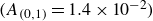
$(A_{(0,1)} = 1.4 \times 10^{-2})$
amplitude cases. The spatial evolution of the energy budget terms, see equation (2.7) applied to the fundamental perturbation, namely production (

$\mathcal{P}_{\beta _{1}}$
), advection (

$\mathcal{T}_{\beta _{1}}$
), viscous effects (

$\mathcal{D}_{\beta _{1}}$
) and the work of nonlinear interactions (

$\mathcal{N}_{\beta _{1}}$
), is depicted in figure 12 for both the flow over the hump and the reference case without hump. The work of perturbation pressure (

$\mathcal{W}_{\beta _{1}}$
) is significantly weaker than the other terms and is therefore neglected from the remainder of the analysis. The discussion of this section is exclusive to the fundamental perturbation, i.e. mode

$\beta = \beta _{1}$
. For the sake of illustration, figure 14 in Appendix A reproduces figure 12 considering mode

$(0,2)$
.
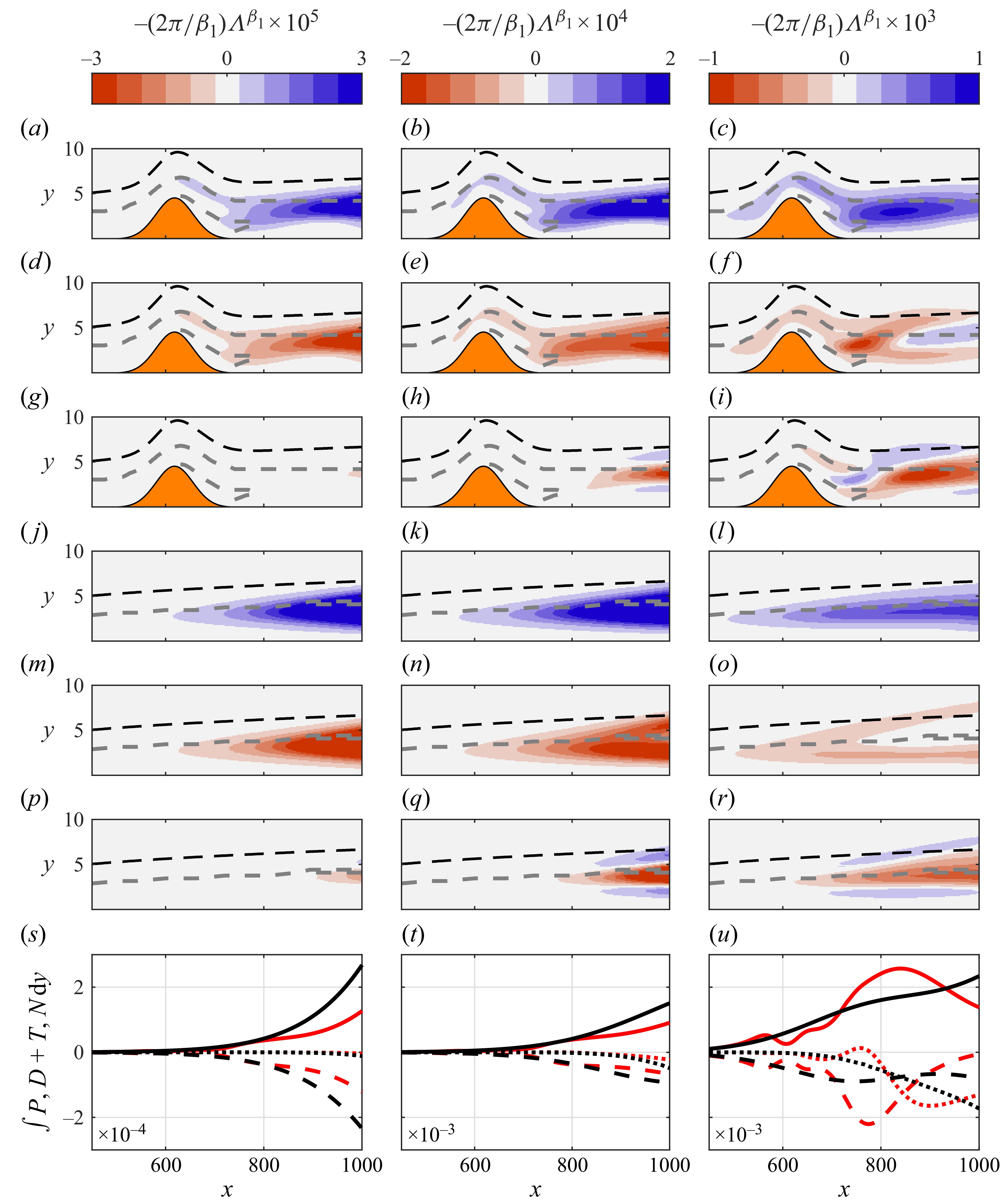
Figure 12. Energy budget distribution (2.7) for the fundamental perturbation,

$\beta = \beta _{1}$
in the (a–i) hump and (j–r) reference case. (a,d,g,j,m,p,s) Low-, (b,e,h,k,n,q,t) medium- and (c,f,i,l,o,r,u) high-
amplitude cases. (a–c, j–l) Production (

$\mathcal{P}_{\beta _{1}}$
) , (d–f, m–o) advection and viscous effects (

$\mathcal{T}_{\beta _{1}} + \mathcal{D}_{\beta _{1}}$
) , and (g–i, p–r) work of nonlinear interactions (

$\mathcal{N}_{\beta _{1}}$
). The black dashed line corresponds to

$\delta _{99}$
. Grey dashed lines indicate loci of crossflow inflection points. (s–u)

$y$
-integrated energy budgets for hump (red) and reference case (black):

$\mathcal{P}_{\beta _{1}}$
(solid lines),

$\mathcal{D}_{\beta _{1}}+\mathcal{T}_{\beta _{1}}$
(dashed lines) and

$\mathcal{N}_{\beta _{1}}$
(dotted lines).
In reference conditions, i.e. without the hump present, a dominant mechanism of linear production drives the spatial amplification of the fundamental CFI until, at least, the virtual location of the hump in all cases considered. This is exemplified by

$\mathcal{P}_{\beta _{1}}$
adding the largest positive (i.e. destabilising) contribution to the energy budget. Considering the low- and medium-amplitude cases, the amplification of the fundamental CFI is linearly dominated until

$x \approx 1100$
and

$x \approx 800$
, respectively; that is, well downstream of the virtual

$x$
-location of the hump. This is substantiated by the agreement between the solutions of linear and nonlinear HNS simulations in the corresponding

$x$
-ranges, as demonstrated in figure 11.
When the hump is present in the low-amplitude case, the mechanism of production maintains a dominant destabilising contribution locally around the hump, i.e.

$\mathcal{P}_{\beta _{1}}$
is the only positive term (figure 12
a). The terms of advection and viscous effects yield a negative contribution (i.e. they are stabilising,
$\mathcal{T}_{\beta _{1}} + \mathcal{D}_{\beta _{1}} \lt 0$
) and thus mainly balance the effect of production, whereas the nonlinear mechanism does not yield a significant contribution to the energy budget. When the amplitude of the incoming CFI is increased in the medium- and high-amplitude cases, the influence of the nonlinear mechanism shortly downstream of the hump appears more evident (figure 12
h,i), albeit it acts mainly stabilising (i.e.

$\mathcal{N}_{\beta _{1}} \lt 0$
). As such, the local CFI destabilisation downstream of the hump for the higher-amplitude cases is ascribed to the enhancement of the mechanism of linear production by the hump (figure 12
u). An opposite trend is observed in the low-amplitude cases. That is, the mechanism of production is weakened by the presence of the hump, when compared with the reference case, which is associated with the decay of CFI amplitude locally after the hump apex, as illustrated in figure 11
Figure 13. Spatial distribution of the lift-up term
$I_2 = -(2\pi /\beta _1)\varLambda ^{\beta _1}_{2}$
(see (2.12)) applied to the fundamental perturbation,

$\beta = \beta _{1}$
. (a,b) Low-, (c,d) medium- and (e,f) high-
amplitude cases for (a,c,e) reference and (b,d,f) hump conditions. The hump is indicated in orange. Dashed black line indicates

$\delta _{99}$
. Cross-flow inflection points are indicated by the white dashed line. Red isolines identify regions exceeding 0.5 and 1 times the maximum contour level.
The analysis further leverages the decomposition of the production term

$\mathcal{P}_{\beta _{1}}$
as outlined in (2.10), (2.12) and (2.13). For all the cases explored in the present work, the term

$I^{\beta _{1}}_2$
(i.e. the lift-up effect) is found to add the main contribution to production, see equation (2.10). The spatial distribution of

$I^{\beta _{1}}_2$
is depicted in figure 13 pertaining to the fundamental mode

$\beta = \beta _{1}$
of the perturbation. In reference conditions, the strength of production increases with the amplitude of incoming CFI, however, no significant qualitative or topological differences are observed in the spatial evolution of

$I^{\beta _{1}}_2$
. In contrast, in the presence of the hump, both the magnitude and spatial topology of

$I^{\beta _{1}}_2$
are significantly altered by the amplitude of the incoming CFI. In the low- and medium-amplitude cases, the strength of

$I^{\beta _{1}}_2$
is notably reduced, as compared with reference conditions. This is particularly evident in the vicinity of the core of the incoming cross-flow vortex, which is approximately following the upper inflectional point in the cross-flow component of the boundary layer (upper white dashed line in figure 13). This reconciles with the trends previously discussed regarding the decay of both production and amplitude of CFI in the same spatial region. However, in the region of cross-flow reversal, delimited by the lower inflectional point (lower white dashed line in figure 13) and further downstream of the hump (
$710\lt x\lt 850$
,

$y\approx 2$
), production is seen to increase locally. This near-wall destabilisation is particularly evident in the high-amplitude case. The emergence of enhanced lift-up and production in the near-wall region can be traced to the outcomes of the linear analysis presented in § 4.1. More specifically, the novel near-wall structure emerging in the region of cross-flow reversal (i.e. lower peak in the double-peak structure in figure 7) carries a strong spatial phase modification, evident as a spanwise shift, compared with the upper body of the incoming CFI perturbation. Such strong modifications in phase have been shown to impart significant changes on the lift-up effect (Casacuberta et al. Reference Casacuberta, Hickel and Kotsonis2024). In addition, the presence of the lower inflectional point in the base flow in combination with the formation of these near-wall structures provide the necessary conditions for rapid spatial perturbation growth near the wall, as predicted by the emergence of a new unstable OS eigenmode in this region (see § 4.2). In the case of high-amplitude incoming CFI, the enhanced near-wall production is able to overwhelm the original incoming perturbation in terms of amplitude, leading to strong stationary structures that can drive transition as discussed in the following section.
5. Concluding discussion
The present work strives to analyse and identify the underlying mechanisms of interaction between stationary CFI and a smooth surface hump. Specifically, the effect of incoming CFI amplitude in the mechanisms of such interaction is investigated. As shown by linear and nonlinear HNS simulations (see figure 11) as well as the experiments of Rius-Vidales et al. (Reference Rius-Vidales, Morais, Westerbeek, Casacuberta, Soyler and Kotsonis2025), whether the hump produces an overall stabilising or destabilising effect appears to be strongly influenced by the amplitude of the incoming CFI intercepting the hump. The combined analysis of pertinent changes on both base flow and perturbation systems covered in the previous sections provides an initial set of principles for these interactions. These principles are to be taken as merely the starting point towards a more holistic understanding since a wealth of key parameters such as Reynolds number, hump shape and CFI wavelength have been kept constant in this work.
The effect of the hump on the laminar base flow is found to manifest as strong modifications in the chordwise and wall-normal velocities, and by association, changes in the boundary layer crossflow component. Crossflow reversal is detected at the leeward side of the hump. Nevertheless, the base flow recovers to the reference case conditions shortly downstream of the hump, in terms of velocity profile and integral quantities. The base flow changes are found to impact the stability of the flow to incoming CFI. These are traced and quantified in this work using local linear stability analysis as well as linear and non-linear HNS simulations.
Energy budgets of the harmonic spanwise-perturbation modes based on the Reynolds–Orr identity are used to evaluate the relative importance of kinetic energy terms, highlighting the dominance of linear production processes. More specifically, the lift-up effect (

$I_2$
) in the vicinity and shortly downstream of the hump was found to dominate the flow. The localised near-wall increase in the

$I_2$
term for all amplitude cases appears to be pivotal towards understanding the destabilisation of CFI in the vicinity of the hump. The spatial region where

$I_2$
experiences a strong increase (

$710\lt x\lt 850$
) corresponds largely to the region in which a secondary near-wall peak was identified in the linear perturbation profiles in figure 7. In the same region, local parallel stability analysis based on the OS equation predicts a strong spanwise deformation and a double-peak shape for the primary unstable mode near the wall. Furthermore, the OS analysis also identifies a short-lived new near-wall mode, emerging purely within the region of cross-flow reversal. Such near-wall structures are, in fact, present in all cases in this work, and are preconditioned in amplitude by the incoming CFI. Considering the above-mentioned observations, a key delineation can be made between beneficial and adverse effects on the transition scenario. Specifically, for medium-to-high CFI amplitudes, this near-wall production dominates local instability growth and leads to the development of highly amplified near-wall structures. Presumably, the strong shears resulting from these structures can provide fertile ground for the development of unsteady secondary instabilities, in a manner similar to the development of type-I and type-II modes in classical saturated CFI (Malik et al. Reference Malik, Li, Choudhari and Chang1999). These in turn can lead to laminar breakdown and accelerated transition observed in the high-amplitude DRE experiments of Rius-Vidales et al. (Reference Rius-Vidales, Morais, Westerbeek, Casacuberta, Soyler and Kotsonis2025). In contrast, for low to medium incoming CFI amplitudes, this near-wall production is present but not strong enough to overtake the overall stabilising effect of the hump on the original incoming CFI. Instead, lasting stabilisation is observed downstream of the hump as a result, which in turn can be linked to the low-amplitude DRE case in the experiments of Rius-Vidales et al. (Reference Rius-Vidales, Morais, Westerbeek, Casacuberta, Soyler and Kotsonis2025), where transition delay was achieved.
While the previous postulation sheds some light onto adverse cases where transition is expected to advance, the origin and nature of the stabilising effect of the hump necessitate further discussion. Pertinent effects can again be traced back to the spanwise deformation of the perturbation system due to the hump. The chordwise region of approximately one hump length downstream of the hump (
$800\lt x\lt 1100$
) appears to play a key role in the stabilisation effect on CFI. This is a region where the spanwise invariant base flow has largely recovered to the reference (i.e. no hump) case (figure 3). As a consequence, a purely modal local stability analysis (i.e. based on OS solutions) in this region indicates an almost identical growth rate as the reference case (figure 7
a). In contrast, the predictions of linear HNS in the same chordwise range and on the same base flow show some differences from the modal solution. This can be further traced to the key component of growth in this region, namely linear production and more specifically the lift-up term

$I_2$
(figure 13). An examination of the constituents of the

$I_2$
term as outlined in (2.13) reveals that under minimal changes in the base flow, the key source of modifications of energy growth must lie in the actual shape of the perturbation. A key impact of the hump on incoming CFI is a strong shearing effect in the spanwise direction. This process is energy-neutral and thus not found in an energy budget analysis. Instead, its effect is visible downstream as lift-up is reduced. The origin of this effect can be largely modelled through a pure spanwise momentum transport of the perturbation shape in a purely advection-based simulation of an incoming CFI perturbation profile. As evident in figures 11 and 7(f), the perturbation entering the recovered base flow region (

$800\lt x\lt 1100$
) is highly distorted due to the aforementioned spanwise shearing effect. In essence, this provides fertile conditions for perturbation growth that is less efficient than a classical non-deformed CFI in this region. In other words, the hump effectively deforms the incoming CFI into a locally less unstable structure.