Sample preparation
The hBN thin flakes were tape-exfoliated from a monocrystalline hBN crystal and transferred onto Si/SiO2 substrates. Then we irradiated the hBN flakes with 2.5 keV 13CO2 (99.0% 13C, Sigma-Aldrich) ions with a dose density of 1012 cm−2 using a home-built ion implanter. The sample is then annealed at 1,000 °C at 10−5 Torr for 2 h to activate the carbon-related defects. For ODMR measurements, we transferred the hBN flakes to a coplanar waveguide using the standard dry transfer method with propylene carbonate stamps. The waveguide is made of 200-nm-thick silver with a 4-nm-thick Al2O3 layer on top.
Sensitivity of a single spin defect
The ODMR contrast varies between defects and can reach as high as 200% (Supplementary Fig. 24). Among the more than 100 spin defects investigated, approximately 25% exhibit a contrast higher than 10%. A single hBN spin defect in our sample has a typical sensitivity of \(5\,\mu {\rm{T}}/\sqrt{{\rm{Hz}}}\) for DC magnetic-field sensing, calculated using \((8{\rm{\pi }}/3\sqrt{3})(1/{\gamma }_{{\rm{e}}})(\Delta \nu /C\sqrt{I})\) (ref. 29), in which Δν is linewidth (20 MHz), C is the contrast (30%) and I is the photon count rate (170 kcts s−1). Furthermore, although most group II and III defects exhibit stable behaviours under a weak laser excitation (≤15 μW), the stability of group I defects varies greatly.
Estimation of nuclear spin polarization
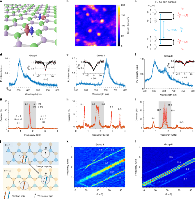
We estimate the polarization of the 13C nuclear spin by evaluating the imbalance between III-2 and III-4 in the ODMR spectrum. The ODMR is taken after the SWAP gate to transfer the electron polarization to the 13C nuclear spin. By using the fitted relative populations of the hyperfine basis states, the polarization can be calculated by the equation
$$P=\frac{{\sum }_{{m}_{I}}{m}_{I}{\rho }_{{m}_{I}}}{I{\sum }_{{m}_{I}}{\rho }_{{m}_{I}}}=\frac{{\rho }_{1/2}-{\rho }_{-1/2}}{{\rho }_{1/2}+{\rho }_{-1/2}}.$$
(2)
Spin readout efficiency
The efficiency of a single-shot spin readout is an important factor to estimate how efficiently we can determine the electronic spin state of a spin defect, which is highly dependent on the defect properties. The readout efficiency is defined by the signal-to-noise ratio from a single readout pulse and can be expressed as38
$${\eta }_{{\rm{s}}}=1/{\sigma }_{{\rm{s}}}={\left(1+2\frac{{\alpha }_{0}+{\alpha }_{1}}{{({\alpha }_{0}-{\alpha }_{1})}^{2}}\right)}^{-1/2},$$
(3)
in which α0 and α1 are the mean numbers of detected photons for a single measurement of the brighter state and darker state, respectively. We estimate the efficiency based on the pulsed ODMR measurements. The pulsed ODMR contrast is 17.5% when we set the readout duration at 5 μs under a PMW = 60 mW microwave drive. The contrast reaches 28% when PMW = 2 W. For each readout laser pulse, we obtain approximately 0.9 photons from the darker state under the 15-μW laser pumping. These yield the efficiency of 0.08 and 0.12 for PMW = 60 mW and PMW = 2 W, respectively. See details in Supplementary Information Section IV.
Gate fidelity
For Rabi oscillations limited by a pure dephasing process, we can write the π-gate fidelity as Fπ = 0.5(1 + exp(−1/Qπ)), in which Qπ = TRabi/Tπ is the quality factor of a π gate39. We extract the coherence time and π-gate time of nuclear spin Rabi by fitting the results in Fig. 3 to the function C(τ) = asin(πτ/Tπ + b)exp(−τ/TRabi) + d, in which C(τ) is the signal contrast of Rabi. As a result, we obtain a Fπ,n = 99.75% π-gate fidelity, with Tπ,n = 0.60 μs and TRabi,n = 117 μs. Similarly, we also estimate the electronic spin π-gate fidelity to be 96.2%, using the same defect and transition in the nuclear spin control experiments.
DFT calculations
We use Quantum Espresso40, an open-source plane-wave software, to perform the DFT calculations. Both the Perdew–Burke–Ernzerhof functional and the Heyd–Scuseria–Ernzerhof hybrid functional (the factor of 0.32 for Fock exchange)41,42 are used for the exchange-correlation interaction. We use the optimized norm-conserving Vanderbilt (ONCV) pseudopotential43,44 for the calculations of excitation energy and the GIPAW pseudopotential45 for the calculation of hyperfine interaction parameters and ZFS. We set the kinetic energy cut-off to be 55 Ry, which is adequate for converging the relevant properties. Geometry optimizations are carried out with a force threshold of 0.001 Ry Bohr−1. We select the 6 × 6 × 1 or higher supercell size of hBN for the calculations of hyperfine parameters and excitation energies. For these calculations, we sample a k-point mesh of 3 × 3 × 1 for the calculation of excitation energies46 and the Γ point for the hyperfine parameters and ZFS28,46. We calculate the zero-phonon line by the constraint occupation DFT method47, the hyperfine parameters using the QE-GIPAW code48, the ZFS by using the ZFS code46 and we cross-compare results between the ZFS code and the PyZFS code49. The key results are summarized in Supplementary Tables 2 and 3.
Simulation of ODMR spectrum
The continuous-wave ODMR spectra shown in Fig. 5 are simulated using the MATLAB toolbox EasySpin50 based on data from the ab initio calculations. EasySpin also takes the nuclear Zeeman and quadrupole interaction into account. Therefore, the continuous-wave ODMR linewidth can be determined according to the hyperfine couplings with the most abundant nuclear-spin-active isotopes: 13C, 11B and 14N. In our simulation, we consider a 13C nuclear spin, ten nearest 11B nuclear spins and two proximate 14N nuclear spins. The other nuclei, located further away, couple more weakly to the electron, scaling with ∝ 1/r3 (in which r is the distance from the central carbon site) and, thereby, have a negligible effect on the ODMR linewidth.
Spin-pair model
The S = 1 transitions are consistently observed alongside the S = 1/2 transitions within the same emitters. To explain the coexistence of both spin transitions in ODMR, we use a weakly coupled spin-pair model32,33 and perform numerical simulations to investigate the underlying mechanism.
Extended Data Fig. 1a provides a simplified representation of the spin-pair model, consisting of two independent defects (defects A and B), separated by ≥1 nm, forming a defect complex. This complex hosts two unpaired electrons that establish different internal charge states depending on their spatial occupancy. When both electrons are localized on the same defect (defect A), they form a closed-shell spin singlet GS with a metastable spin triplet state (S = 1), which can be accessed through laser excitation and intersystem crossing transitions (left panel in Extended Data Fig. 1b). This state corresponds to a strongly coupled spin-pair charge state and explains the S = 1 transitions.
Alternatively, laser excitation can induce charge hopping that transfers one electron from defect A to defect B, forming a weakly coupled defect pair. In this configuration, each defect hosts a single electron (S = 1/2), as illustrated in the right panel of Extended Data Fig. 1b. This spin-dependent charge hopping yields a corresponding spin-dependent PL signal32.
The actual GS, which is also the optically active state, is determined by the lowest-energy charge configuration and depends on the specific defect species and the local Fermi energy level. We considered two possible energy-level configurations (Supplementary Information Section XII), with Extended Data Fig. 1c depicting the most likely scenario. In the most stable charge state, both electrons occupy the same defect site, yielding a S = 0 GS and a metastable S = 1 state. Laser excitation can then generate a metastable spin-pair charge state by promoting transitions from the S = 1 to the S = 1/2 manifold. The pronounced asymmetry in the Rabi oscillations, reflected by an increasing contrast baseline in both S = 1/2 and S = 1 transitions, strongly supports the metastable nature of these spin manifolds.
In the presence of a 13C nuclear spin, the defect electron spins can couple to the nuclear spin through hyperfine interactions, which vary across different charge states. In the weakly coupled spin-pair state, the nuclear spin is primarily coupled to a single electron spin at defect A. This is consistent with our experimental observations, in which hyperfine coupling constants Azz of 130 and 300 MHz were measured for group II and group III defects, respectively.
Given their distinct hyperfine features, group II and III defects are likely to have more well-defined and deterministic structures. By contrast, group I defects, lacking hyperfine splitting, may include a range of chemical configurations: either similar to group II and III defects (but involving 12C instead of 13C) or very different chemical structures. This structural variability may account for the broader range of stability observed in group I defects, whereas group II and III defects tend to exhibit more consistent and stable behaviour under experimental conditions.
Simulation of spin photodynamics
On the basis of the possible energy-level models, we numerically simulate the spin photodynamics using the Lindblad master equation:
$$\dot{\rho }=-\,i[H,\rho (t)]+\sum _{k}{\varGamma }_{k}\left[{L}_{k}\rho (t){L}_{k}^{\dagger }-\frac{1}{2}\{{L}_{k}^{\dagger }{L}_{k},\rho (t)\}\right],$$
(4)
in which ρ(t) is the time-dependent density matrix, Γk represents transition rates and Lk are the associated Lindblad operators. This simulation allows us to predict PL signals in both continuous-wave ODMR and pulsed Rabi experiments (see details in Supplementary Information).
In the continuous-wave ODMR simulation, we use the full Hamiltonian, which includes the optical manifold, spin-pair states and spin-triplet states. For model 1, in which the GS is a spin singlet (S = 0), the Hamiltonian is written as:
$$H={H}_{{\rm{pair}}}\oplus {H}_{m,S1}\oplus {H}_{{\rm{eg}}}=\left(\begin{array}{ccc}{H}_{{\rm{pair}}}^{8\times 8} & & \\ & {H}_{m,S1}^{6\times 6} & \\ & & {H}_{{\rm{eg}}}^{4\times 4}\end{array}\right)$$
(5)
in which Heg, Hm,S1 and Hpair describe the optical manifold, the spin S = 1 metastable state and the spin-pair state, respectively (see detailed expressions in Supplementary Information). For each subspace, we consider a 13C nuclear spin coupled through hyperfine interaction. The full Hamiltonian is a direct sum of individual spin manifolds, meaning that there is no coherent interaction between them. Instead, they are connected by means of incoherent transitions described by the Lindblad operators Lk.