Study population: the UK Biobank
The UK Biobank (UKBB) recruited 503,000 community-based adult volunteers aged 40-69 from 2006-2010 in 22 study centers across the United Kingdom: England, Wales, and Scotland18. In the current analysis, we evaluate the UKBB imaging subgroup of 41,212 participants who returned between 2014-2020 to undergo spinal dual-energy X-ray absorptiometry (DXA) assessment (Lunar iDXA densitometer; GE Healthcare, Chicago, Illinois). At the baseline visit, extensive demographic and biometric information were collected including age, race, smoking status, height, and weight via questionnaires and physical measurements. The Townsend Deprivation Index (TDI), a composite measure for socioeconomic status calculated from unemployment, car and home ownership, and household crowding status, was evaluated from self-reported metrics19. Additionally, blood was collected for serum biomarker and genomic analyses. Information on prior disease conditions were derived from baseline data and clinical data aggregated across healthcare providers: the Health Episode Statistics database from England, Patient Episode Database for Wales, and the Scottish Morbidity Record 01 for Scotland. The International Classification of Diseases, Tenth Revision (ICD10) was used.
This study was approved by the North West Multi-Centre Research Ethics Committee (MREC) and informed consent was collected from all participants. Further information on the study design of the UKBB has been previously published18.
Machine learning
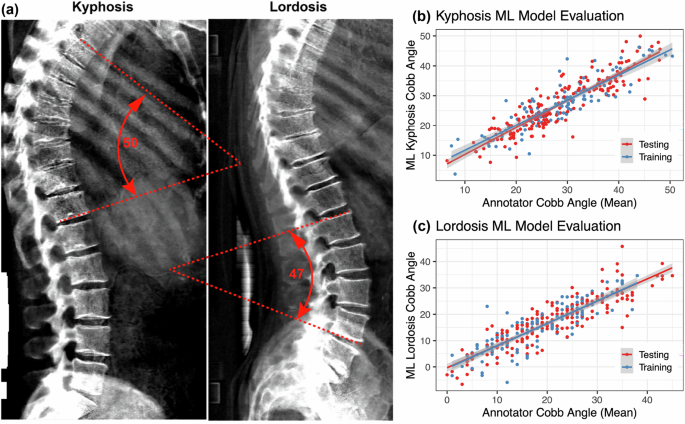
Detailed methods are available in the Supplementary Machine Learning Methods document. In brief, we constructed an image-processing pipeline that (1) establishes a trace along the center of the vertebral column, (2) identifies an appropriate thoracic or lumbar section of the spine for analysis of kyphosis or lordosis, respectively, and (3) measures the angle difference between lines tangential to the spinal traces at the top versus bottom of that section as a proxy for the Cobb angle (Supplemental Fig. 12). For kyphotic angle, the thoracic spine approximately above and including vertebra T12 was analyzed. For lordotic angle, the lumbar spine approximately between and including vertebrae T12 through L5 was analyzed. Full details can be found in the Supplementary Methods and GitHub repository (https://github.com/graham-calico/KyphoLordoDxa.git). Kyphosis and lordosis were measured using the python tool “spineCurve.py”. The following command-line options were invoked, for kyphosis: “–aug_flip –side_facing right”; and for lordosis: “–lumbar –aug_flip –side_facing right –aug_tilt 0.5”. Exact reproduction of the results in this manuscript should additionally invoke the “–legacy” flag. Further methods are described in Supplementary Machine Learning Methods.
Statistical analyses
For all analyses, two-tailed P-values were calculated. Significance was defined as a false discovery rate-corrected p-value (pFDR)
We assessed participant characteristics at the time of the imaging visit, stratified for presence and absence of hyperkyphosis (>40°) and hyperlordosis (>30°). Continuous variables were summarized as medians and interquartile ranges (IQR), and categorical variables were presented as counts and percentages. The correlation between kyphotic and lordotic angles was displayed using locally smoothed regression with span = 0.75 and the correlation coefficient (r) was calculated using Pearson product-moment correlation after confirming the linearity assumption could be reasonably met. Unadjusted Wald maximum likelihood estimation was used to calculate the risk ratio between prevalent hyperkyphosis and hyperlordosis.
To evaluate the association between age and kyphosis/lordosis angles, several analyses were conducted. First, the sex-stratified association between age and each kyphotic and lordotic angle was plotted using locally smoothed regression (span = 0.75) with 95% confidence intervals (ggplot2). Second, participants were binned by age decile (e.g. 45-54, 55-64, etc.), and the proportion of individuals in each respective age category that had high kyphosis (40° to 50°+) and lordosis (30° to 40°+) angles by 5° intervals was graphed. Last, the mean age of participants in each 10° kyphosis by lordosis angle was presented as a heatmap.
To gain further insight into factors that might contribute to increased spinal curvature, we used multivariable linear regressions to evaluate the association of Cobb angles with 414 pre-existing medical conditions with prevalence > 200 in our population, 59 clinical chemistry measures, and 15 body measure traits (adiposity, bone mineral density, muscle, lung traits) in UK Biobank. All associations were adjusted for age, age², sex, age*sex, smoking, BMI, and Townsend deprivation index. FDR-adjusted significant associations between Cobb angle (either kyphosis or lordosis) and pre-existing conditions and clinical chemistry measures were presented. All 15 adiposity and skeletal-muscular body measure associations were presented, regardless of significance since they were related to our main study interest of phenotypic body composition associations with kyphosis and lordosis angle. All these skeletal-muscular associations were adjusted for variables listed above except BMI was not included in the adjustment of measures highly collinear with BMI calculation (BMI, height, total fat mass, and visceral adipose tissue).
We expected that the associations of various musculoskeletal traits on spine curvature could be non-linear. Thus, to assess ranked independent predictors of Cobb angles (out of body measure traits, age, sex, and smoking status), we ran variable selection using a 10-fold cross-validated boosted generalized regression model with interaction depth = 2 and modeled selected features using splines in the generalized additive model (GAM)20. Variables with relative influence > 0 were selected for the model and relative variable influence percentages were presented. In secondary analyses, we reran all these linear regressions after stratifying by sex to examine potential effect modification by sex of these associations.
Genetic analyses
UKBB imputed genotypes were used in all genetic analyses17. Further details on their methods have been previously published (https://biobank.ndph.ox.ac.uk/showcase/showcase/docs/impute_ukb_v1.pdf). We excluded SNPs with (1) minor allele frequency 10%, or (4) demonstrated deviation from Hardy-Weinberg equilibrium (HWE p −10). Participants were excluded from the genomics analyses if they were (1) not of European ancestry (field ID 22006), (2) had heterozygosity or genotype call rate outliers (field ID 22027), (3) demonstrated sex chromosome aneuploidy (field ID 22019), (4) had a mismatch between genetic sex and self reported sex (field ID 22001), or (5) were genetically related (field ID 22011). This yielded a total of 9,911,384 SNPS and 33,413 participants in the genetic analyses. Bonferroni correction was used to evaluate significance in all the genetics analyses and a threshold of pFDR
Genome wide association study
For the initial genetic wide association study (GWAS), a whole-genome regression model was conducted on kyphosis and lordosis separately using REGENIE, a computationally efficient, machine learning-based parallel analysis approach21. In brief, REGENIE first uses cross-validated ridge regression by SNP block for dimension reduction of the genetic data. Then, a second cross-validated ridge regression for each trait is conducted to combine predictors from the first ridge regression into an overall prediction by trait, which is then decomposed by chromosome for a leave-one-chromosome-out (LOCO) scheme. These LOCO predictors are used as a covariate where each phenotype is tested by the set of imputed SNPs, also adjusting for genotype SNP chip (Illumina vs Affymetrix), sex, age, age2, age*sex, and recruitment center. We verified that the test statistics showed no inflation compared to the expectation using the genomic control lambda coefficient (1.13 for kyphosis and 1.09 for lordosis) and the intercept (0.999, SD 0.009 for kyphosis and 1.000, SD 0.084 for lordosis) of linkage disequilibrium score regression.
Multi-trait analysis of GWAS (MTAG)
The method for conducting MTAG from GWAS statistics has been previously described22. MTAG enhances statistical power by leveraging the genetic correlation between traits to generate trait-specific estimates for each SNP. Based on linkage disequilibrium score regression (LDSC) estimates of genetic correlations between kyphosis and lordosis, a joint analysis of the two traits using the GWAS summary statistics was conducted using MTAG. Briefly, variants were restricted to those with minor allele frequency (MAF) > 0.01, and those that passed quality control (QC) in the individual trait GWAS. We verified that MTAG results were not inflated compared to the expectation using the genomic control lambda coefficient (1.14 for kyphosis and 1.11 for lordosis) and the intercept (0.998, SD 0.0085 for kyphosis and 0.9842, SD 0.0089 for lordosis) of LDSC.
Genetic correlation and heritability
To examine if the genetic variation linked to spine angles shares genetics with other traits, we calculated genetic correlations with GWAS catalog phenotypes for kyphosis and lordosis, respectively. All available summary statistics from the EBI GWAS catalog (www.ebi.ac.uk/gwas/) were downloaded on October 19, 202223. Of the 25,475 summary statistics files, 20,021 could be successfully re-formatted by the munge step of LDSC24. Of those, LDSC calculated a positive heritability for 14,843 summary statistics files. Of these traits, 10,170 and 10,138 for kyphosis and lordosis, respectively, yielded non-null SNP heritabilities and were used for downstream genetic correlation analysis.
In addition to traits available on the EBI GWAS catalog, we also estimated the heritability of and genetic correlations between kyphosis or lordosis angles with musculoskeletal traits measured in the UKBB (adiposity, bone mineral content, muscle and lung traits). LDSC was calculated using the repository at https://github.com/bulik/ldsc/, version aa33296. We estimated genetic correlation and heritability using default parameters and the –rg command and –h2 command, respectively (example: ldsc.py –rg kyphosis.sumstats.gz, lordosis.sumstats.gz –ref-ld-chr eur_w_ld_chr/ –w-ld-chr eur_w_ld_chr/ –out). Allele polarization was pre-harmonized to match the reference file w_hm3.snplist. Analyses were adjusted for sex, age, age², age*sex, and recruitment center.
Fine-mapping
GCTA was used for approximate conditional analysis25,26. We considered all variants that passed QC (above) and were within 500 kb of the index variant, except in the major histocompatibility complex (MHC) region due to the complex linkage disequilibrium (LD) structure of the region (GRCh38::6:28,510,120-33,480,577)27. For the LD calculation reference panel, we used genotypes from 5,000 randomly-selected, unrelated, Northern European UKBB participants. For individual loci, variants with locus-wide evidence of association (pjoint 6) were considered conditionally independent. A threshold of p 8 was used as the genome-wide association threshold for defining a locus.
Construction of genetic credible sets
For every distinct GWAS signal, credible sets were calculated at a threshold of 95% probability of containing at least one variant with a true non-zero effect size. First, the natural log approximate Bayes factor, Λj, was computed for the jth variant within the fine-mapping region:
$${\varLambda }_{j}={\mathrm{ln}}\left(\sqrt{\frac{{V}_{j}}{{V}_{j\,+\omega }}}\right)\frac{\omega {\beta }^{2}}{2{V}_{j}({V}_{j}+\omega )}$$
(1)
where βj and Vj are the estimated effect size and corresponding variance, respectively28. The parameter ω denotes the prior variance in allelic effects and is estimated as (0.15σ)2, where σ is the standard deviation of the phenotype. This standard deviation (σ) was estimated using the formula below:
$$2{n}_{j}{f}_{j}(1-{f}_{j})\sim {\sigma }^{2}\frac{1}{{Var}({\beta }_{j})}-1$$
(2)
Here, Var(βj) is the variance of the beta coefficients, fj is minor allele frequency, nj is sample size, and σ2 is the coefficient of the regression which was used to estimate σ with \(\sigma =\sqrt{{\sigma }^{2}}\).
In genetic loci with multiple distinct association signals, we used two techniques (1) exact conditional analysis adjusting for all other index variants in the fine-mapping region and (2) marginal analysis not adjusting for other index variants within the locus. In genetic loci with only a single association signal, we used an unconditional meta-analysis.
Given l variants in the region, we then calculated the posterior probability, πj, that the jth variant was driving the association using:
$${\pi }_{j}=\frac{(1-\gamma ){\varLambda }_{j}}{l{\sum }_{k=0}^{l}{\varLambda }_{k}}$$
(3)
where γ denotes the prior probability for no association at this locus and k indexes the variants in the region (with k = 0 indicating no association in the region). To account for the expected false discovery rate of 5%, we set γ = 0.05 since a threshold of pmarginal −8 was used to identify loci for fine-mapping.
For each signal, the 95% credible set was then constructed by (1) ranking all variants by their Bayes factor and (2) including all ranked variants until their cumulative posterior probability exceeded 0.99.
PheWAS
Fine-mapped lead SNPs were annotated to potential functional genes using the Ensembl Variant Effect Predictor, Open Targets, and dbSNP databases. We also considered previous significant associations in the GWASAtlas catalog and summarized our findings in Table 1.
Table 1 Genetic associations between phenotypic traits and kyphosis and lordosis angleColocalization
We performed colocalization tests to evaluate whether two traits (spine angle and gene expression) share the same underlying causal variants. For gene expression colocalizations, we used summary statistics from GTEx v829. For physiological and disease trait colocalizations, we used UKBB summary statistics of standardized quantitative and ICD10-categorized traits30. We identified UKBB phenotypes where the minimum p-value within the +/−500kb region around the SNP locus was -8. Colocalization analysis was conducted using the coloc R package with default priors and including all variants within 500 kb of the index variant31. Two genetic signals were considered to have strong colocalization evidence if PP3 + PP4 ≥ 0.99 and PP4/PP3 ≥ 5 and suggestive colocalization evidence if PP3 + PP4 ≥ 0.8 and PP4/PP3 ≥ 331.
Mendelian randomization analysis
To further evaluate causal associations between the genes identified and spinal curvature, we conducted MR analyses32. In MR analysis, we used cis-regulatory or splicing variants that affect RNA expression and function of implicated genes as instrumental variables. We evaluated whether these expression and splicing changes drive changes in a phenotype of interest. Since genetic variants are theoretically randomly assigned when passed from parents to offspring, this method is expected to minimize the effect of confounding and avoids reverse causation.
The MR method relies on three important assumptions: (i) the genetic variant is associated with the exposure, (ii) the genetic variant is not associated with any confounders, (iii) the genetic variant is not associated with the outcome through any pathway other than via the exposure (no horizontal pleiotropy). Since multiple tissues can affect spine curvature, we carried out two sample MR analyses across all 54 tissue types measured in GTEx v829. To identify independent SNP instruments for each exposure, we pruned GWAS-significant SNPs (p-value -8) for each risk factor using a threshold of r2
For sensitivity analyses, the MR analysis was also reconducted using (1) MR-Egger regression and (2) weighted median-based and mode-based tests of the ordered Wald ratio estimates33,34. Since weighted median and mode estimates assume that the estimates from pleiotropic variants are outliers, these methods tend to be less sensitive to the effect of pleiotropic variants35. On the other hand, MR-Egger involves a weighted linear regression to evaluate the marginal effect of each SNP on the outcome on the marginal effect of each SNP to the exposure. Thus, this method evaluates the overall directional pleiotropic contribution of weak instrumental SNPs on the risk estimate. As such, we used these methods as sensitivity analyses to confirm that there was a consistent directional effect between the variants and traits relative to the IVW and Wald ratio results35.
Reporting summary
Further information on research design is available in the Nature Portfolio Reporting Summary linked to this article.