The micro-canonical ensemble is commonly defined as the maximally mixed state-supported in a narrow window around a fixed energy. This physically models maximal uncertainty with an energy constraint. However, arbitrary and even physically motivated states, such as low-entanglement states, can have non-trivial support over the whole spectrum during the whole time evolution; these states will, therefore, never be micro-canonical in the sense above, particularly not at equilibrium. With the goal of overcoming this issue, we leverage techniques used to prove equivalence between micro-canonical and canonical ensembles. Such equivalence results have a long history, with the first proofs for lattice systems in the strict thermodynamic limit being given by Lima44,45; later, Brandão and Cramer26 generalized this to finite-sized lattice systems. In this latter work, it is proven that equivalence with a canonical ensemble is already achieved by states confined in a micro-canonical window that are not maximally mixed but have sufficiently high entropy and an expected energy that is sufficiently close (but not necessarily equal to) the expected energy of the Gibbs state. We adapt this result to the situation in which the state is not confined to a window but instead has support over many such windows, plus decaying tails. First of all, we call this a generalized micro-canonical ensemble, meant to capture the thermal behavior of states that are supported on regions of the spectrum larger than what the usual micro-canonical ensemble allows.
Definition 1
(Generalized micro-canonical ensemble (GmE)) Let [E − Δ, E + Δ] (Δ > 0) denote an energy window centered around a value E and divided into K bins of various size δk, with k = 1, …, K. Let δ = (δ1, …, δK); we define a generalized micro-canonical ensemble (GmE) to be the state of the form
$$\omega := \omega (E,\Delta ,\delta ,{{\bf{q}}})=\sum _{k=1}^{K}{q}_{k}{\omega }_{{\delta }_{k}}$$
(6)
where \({\omega }_{{\delta }_{k}}\) is the micro-canonical ensemble supported inside the window k, and where q = (q1, …, qK) such that \({\sum }_{k = 1}^{K}{q}_{k}=1\).
This state, therefore, physically represents a statistical combination of micro-canonical ensembles; see Fig. 2. For the sake of simplicity, we will choose δk = δ from now on. However, all results are shown in the Supplementary Information with this assumption relaxed, unless otherwise specified. Before stating our first main result, we need to introduce the notion of the Berry-Esseen (BE) error, which quantifies the difference between a state written in the energy eigenbasis and a Gaussian distribution. More specifically, if Πx is the projector onto all energy eigenstates with energy smaller than x, then the BE error of ρ with respect to H is defined as \({\zeta }_{N}=\mathop{\sup }_{x}| {{\rm{tr}}}\left(\rho {\Pi }_{x}\right)-G(x)|\), where G(x) is the Gaussian distribution with the same mean and variance as ρ. It was proven that if ρ has exponential decay of correlations, then \({\zeta }_{N}\le \tilde{O}({N}^{-1/2})\)26. Simple examples of saturating this bound are known, and this bound is expected to be saturated by certain non-thermalizing models. Nonetheless, under some more generic constraints, such as highly entangled eigenstates, a more favorable scaling is expected, even up to ζN ≤ e−Ω(N) for product states46. From now on, we denote by ζN the BE error with ρ = gβ(H). In what follows, we will assume \({\zeta }_{N}\le \tilde{O}({N}^{-1/2-\kappa })\) for some κ ≥ 0. This includes the worst case κ = 0.
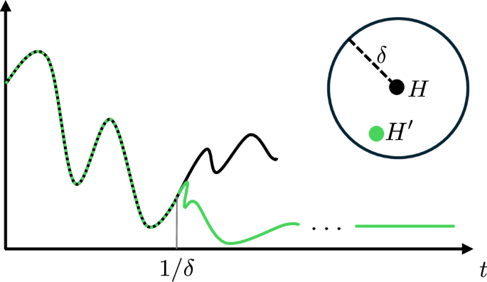
Fig. 2: Cartoon illustration of the setting of Definition 1 and Definition 2.
In this example, the state is diagonal in the energy eigenbasis, and it is represented as a probability distribution. The blue line is a Generalized microcanonical Ensemble (GmE) state, and the green line an approximate GmE state. The insert shows both states restricted to one of the windows.
Theorem 1
(Ensemble equivalence) Let H be a local Hamiltonian and β an inverse temperature for which the Gibbs state gβ(H) has exponential decay of correlations, standard deviation \(\sigma \ge \Omega (\sqrt{N})\) and Berry-Esseen error \({\zeta }_{N}\le \tilde{O}({N}^{-1/2-\kappa })\) for κ ≥ 0. Let ω denote a GmE with Δ, δ satisfying
$${{{\rm{e}}}}^{{\Delta }^{2}/{\sigma }^{2}}\le \tilde{O}\left({N}^{\frac{1-\alpha }{D+1}}\right),\quad \Omega \left({N}^{\frac{1-\alpha }{D+1}-\kappa }\right)\le \delta \le \sigma ,$$
(7)
with α ∈ [0, 1) and such that ∣E − Eβ∣ ≤ σ. Then for any side length l such that \({l}^{D}\le {C}_{1}\,{N}^{\frac{1}{D+1}-{\gamma }_{1}\alpha }\), the following holds
$${D}_{l}(\omega ,{g}_{\beta }(H))\le {C}_{2}{N}^{-{\gamma }_{2}\alpha },$$
(8)
with C1, C2 being system-size independent constants, and γ1, γ2 only depend on the dimension of the lattice D.
This first main result shows that, for appropriate choices Δ and δ, GmE states are locally indistinguishable from Gibbs states. A GmE state can be seen as a mixture of micro-canonical states spanning a range of temperatures and Theorem 1 shows that as long as its range is small enough, the state still looks thermal with a well-defined temperature. Notice that if κ > 0, i.e., if the BE error is better than the worst case scenario, δ can be chosen to decay with the system size. This window size will play a crucial role in determining the minimal “strength” of the randomization necessary to enforce thermalization; our bounds on δ are inherited from the techniques of ref. 26. It is worth noting that later works significantly improved this window size for the equivalence of the canonical and micro-canonical ensemble, up to sizes \(\delta \sim {{{\rm{e}}}}^{-\sqrt{N}}\)47,48, but these results are either dependent on an exactly micro-canonical state (with maximum entropy) or on the micro-canonical state having an exactly defined energy, which makes their application for our purposes difficult.
Keeping in mind our initial goal of capturing equilibrium states resulting from natural and physically motivated initial states, it may seem artificial to consider only block-like states with sharp jumps between energy intervals. Therefore, postponing the discussion about their physicality to the next Section below, we, first of all, prove that the same ensemble equivalence holds if the state’s structure gets more relaxed, i.e., if it is only approximately GmE in a sense precisely elucidated below.
Definition 2
(Approximate GmE) Let E, Δ, δ, q be as in Definition 1. We define ωη an approximate GmE if it is of the form
$${\omega }_{\eta }={p}_{\Delta }\left(\sum _{k=1}^{K}{q}_{k}{\tilde{\omega }}_{{\delta }_{k}}\right)+(1-{p}_{\Delta }){\rho }_{{{\rm{tail}}}}$$
(9)
and its von Neumann entropy satisfies
$$\sum_{k=1}^{K}{q}_{k}(S({\omega }_{{\delta }_{k}})-S({\tilde{\omega }}_{{\delta }_{k}}))\le \eta ,$$
(10)
with \({\tilde{\omega }}_{{\delta }_{k}}\) being defined on the Hilbert space spanned by the eigenstates in the k-th energy bin, and ρtail on the Hilbert space spanned by the eigenstates outside [E − Δ, E + Δ].
This state represents a more physical version of a GmE state inside the energy window Δ, with decaying tails outside, that has an entropy η-close to the maximum one. Importantly, in Supplementary Note 1, we demonstrate that Theorem 1 holds true also for the approximate GmE and takes the form
$${D}_{l}({\omega }_{\eta },{g}_{\beta }(H))\le {C}_{2}{N}^{-{\gamma }_{2}\alpha }+2(1-{p}_{\Delta }),$$
(11)
with \(\eta \le {N}^{\frac{1-\alpha }{D+1}}\).
This shows that states that are concentrated around an energy regime and are sufficiently “smooth” are locally equivalent to Gibbs states. The results above are a generalization of the equivalence of ensembles result of ref. 26, and their proof is presented in Supplementary Note 1.
The next question is whether (approximate) GmE states can actually be obtained from the Hamiltonian evolution of isolated systems under natural or typical conditions. There are two main aspects we consider when talking about “natural” conditions: (i) the Hamiltonian responsible for the time evolution and (ii) the initial state of the system. Regarding (i), we consider typical Hamiltonians in the sense that we will make precise below in order to exclude edge cases or fine-tuned Hamiltonians for which one does not expect thermalization (for instance, integrable models). Concerning (ii), previous typicality approaches have assumed the initial state to be confined in a well-defined energy interval, and have shown properties of the relaxation towards a micro-canonical ensemble in said interval. Here, instead, we start from the assumption of exponential decay of correlations, i.e., low entanglement between spatially separated regions, which we take as natural starting states for lattice systems. These states have been shown to have fast decaying tails in energy49 which makes them ideal candidates to flow to approximately GmE states. Here, for simplicity of presentation, we focus on the case of product states and leave the more general case of states with exponential decay of correlations and the proofs to Supplementary Note 3.
Let us expand on the ensemble of typical Hamiltonians that we consider. Starting from any local Hamiltonian on the lattice, we divide its energy spectrum into energy intervals of equal width δ which we call Ik, for k = 1, ⋯ , K. The eigenstates contained within each interval span a vector space which we call \({{{\mathcal{W}}}}_{k}\). We then consider unitaries of the form U = ⨁kUk, where Uk is drawn from the Haar measure of the unitary group acting on \({{{\mathcal{W}}}}_{k}\). This defines an ensemble of random unitaries which we denote as \({{\mathcal{E}}}(\delta )\). A typical Hamiltonian is then UHU† for such a random unitary U. All these Hamiltonians have the same spectrum as the original local Hamiltonian H, and the randomization given by U is designed to preserve the expected energy of any state.
The following is a consequence of measuring concentration and the results of ref. 49 about the energy tails of product states.
Lemma 1
(Approximate GmE at equilibrium) Let ρ be a product state and H be a local Hamiltonian. Let \({\rho }_{\infty }^{UH{U}^{{\dagger} }}\) be defined as in Eq. (1), where U is drawn from \({{\mathcal{E}}}(\delta )\). Consider the interval I = [E − Δ, E + Δ] around \(E={{\rm{tr}}}\left(\rho UH{U}^{{\dagger} }\right)\) with \(\Delta \ge \omega (\sqrt{N})\) an integer multiple of δ, then
$${\rho }_{\infty }^{UH{U}^{{\dagger} }}={p}_{\Delta }\left(\sum_{k:{I}_{k}\subset I}{q}_{k}{\tilde{\omega }}_{{\delta }_{k}}\right)+(1-{p}_{\Delta }){\rho }_{{{\rm{tail}}}}$$
(12)
with \({p}_{\Delta }\ge 1-{{{\rm{e}}}}^{-{c}_{1}\frac{{\Delta }^{2}}{N}}\), and for r > 0, with probability at least 1 − 2−r+1, we have
$$\sum_{k:{I}_{k}\subset I}{q}_{k}(S({\omega }_{{\delta }_{k}})-S({\tilde{\omega }}_{{\delta }_{k}}))\le r,$$
(13)
where c1 is a system-size independent constant.
We have then the following consequence on typical thermalization.
Theorem 2
(Typical thermalization) Let H be a k-local Hamiltonian and ρ be a product state. Let gβ(H) be the Gibbs state of H at inverse temperature β such that \(| {{\rm{tr}}}({g}_{\beta }(H)H)-{{\rm{tr}}}(\rho H)| \le \sigma\). Assume gβ(H) has exponential decay of correlations, \(\sigma \ge \Omega (\sqrt{N})\), and \({\zeta }_{N}\le \tilde{O}({N}^{-1/2-\kappa })\). For any constant α ∈ [0, 1), choosing \(\delta =\Omega ({N}^{\frac{1-\alpha }{D+1}-\kappa })\), with probability at least \(1-\exp (-{c}_{2}{N}^{\frac{1-\alpha }{D+1}})\) drawing U at random from \({{\mathcal{E}}}(\delta )\), we have
$${D}_{l}({\rho }_{\infty }^{UH{U}^{{\dagger} }},{g}_{\beta }(H))\le {C}_{2}\,{N}^{-{\gamma }_{2}\alpha }+\tilde{O}\left({N}^{-{\gamma }_{3}(1-\alpha )}\right),$$
(14)
where c2, C2, γ2, γ3 are system-size independent constants.
In Supplementary Note 3, we state and prove these results more generally for any state concentrated around its average, which includes states with exponentially decaying correlations. The consequence of this relaxation of the assumption is that the decay in the system size is quasi-polynomial rather than polynomial. We stress that we pick the specific case of low-entanglement states because their fast decaying tails allow for better approximation when the tails are cut outside of the window of size Δ. As a matter of fact, our results hold for any state ρ, as long as its energy variance is linearly bounded \({\sigma }_{\rho }^{2}={{\rm{tr}}}\left(\rho {H}^{2}\right)-{{\rm{tr}}}{\left(\rho H\right)}^{2}\le O(N)\). We could then use Markov’s inequality as opposed to the concentration bounds in49 to show a linear decay of the tails in \({\Delta }^{2}/{\sigma }_{\rho }^{2}\). Since for Theorem 1 to apply, we must have \({\Delta }^{2}/{\sigma }_{\rho }^{2} \sim \log (N)\), this leads only to bounds decaying very slowly as \(\sim 1/\log (N)\) in Theorem 2. Theorem 2 shows that the equilibrium state is locally thermal; in the Supplementary Note 3 we show under mild spectral assumptions that the randomized Hamiltonian equilibrates with high probability to this state. Although it may seem strange at first glance that under the dynamics of UHU† the state thermalizes to the Gibbs state of H and not of UHU†, we prove that the Gibbs states of these two Hamiltonians are locally indistinguishable. More specifically, under the same assumptions as Theorem 2, for any U drawn from \({{\mathcal{E}}}(\delta )\) we have
$${D}_{l}({g}_{\beta }(H),{g}_{\beta }(UH{U}^{{\dagger} }))\le O({N}^{-{\gamma }_{4}\alpha -{\gamma }_{4}\kappa })$$
(15)
for system-size independent constants γ4, γ5. The proof may be found in the Supplementary Note 3, and easily generalizes to other choices of δ. On an intuitive level, this can be seen because both states are locally indistinguishable from a micro-canonical state, which is the maximally mixed state inside an energy window and, hence, invariant under rotations in the window. As anticipated, the unitary ensemble \({{\mathcal{E}}}(\delta )\) is chosen in order to approximately preserve the energy of any state; this implies that \(U \sim {{\mathcal{E}}}(\delta )\) approximately commutes with the Hamiltonian, and we show ∥H − UHU†∥∞ ≤ δ. For the choice of δ as in Theorem 2, we derive the following result
$$\parallel {{{\rm{e}}}}^{-iHt}\rho {{{\rm{e}}}}^{iHt}-{{{\rm{e}}}}^{-i{H}^{{\prime} }t}\rho {{{\rm{e}}}}^{i{H}^{{\prime} }t}{\parallel }_{1}\le 2t\,O\left({N}^{\frac{1-\alpha }{D+1}-\kappa }\right),$$
(16)
with \({H}^{{\prime} }=UH{U}^{{\dagger} }\). This means that the dynamics under H and UHU† are indistinguishable up to a time \({t}^{* } \sim {N}^{\kappa -\frac{1-\alpha }{D+1}}\). If κ > 0, that is, the BE error decays faster than the worst-case scenario, α can be chosen such that t* increases with the system size. In other words, H and UHU† generate nearly the same dynamics for a time t* ~ poly(N). Finally, we would like to emphasize that our rigorous approach allows us to put on precise and solid ground some of the results obtained on equilibration in ref. 50.
It is now worth noting that if both ρ and σ are translation-invariant, the averaging over regions in the definition of Dl(ρ, σ) can be dropped, making the indistinguishability statement valid for any observable supported on an individual small region. We show that if the original Hamiltonian is translation-invariant, we recover this property to some extent in the equilibrium state of the perturbed Hamiltonian. More specifically, consider an observable A supported in \(C\in {{{\mathcal{C}}}}_{l}\) and H translation-invariant. For U drawn from, \({{\mathcal{E}}}(\delta )\) we show, assuming all windows centered around an extensive energy contain exponentially many eigenvalues, that except with probability e−Ω(N),
$$\begin{array}{l}\left | {{\rm{tr}}}\left(\left({g}_{\beta }(H)-{\rho }_{\infty }^{UH{U}^{{\dagger} }}\right)A\right)\right | \le \\ {{{\rm{e}}}}^{-\Omega (N)}+{D}_{l}\left({\rho }_{\infty }^{UH{U}^{{\dagger} }},{g}_{\beta }(H)\right).\end{array}$$
(17)
Details and proofs are available in the Supplementary Note 5. By applying this to ρ = gβ(UHU†) we also get translation invariance in the same sense for the randomized Gibbs state, that is, \({\rho }_{\infty }^{UH{U}^{{\dagger} }}\) can be replaced by gβ(UHU†) in Eq. (17).
Turning to notions of dynamical thermalization, we now investigate the typical time-evolution of the expectation value of a generic observable A, \({\langle A\rangle }_{\rho }:= {{\rm{tr}}}\left(A\rho \right)\), under the evolution generated by UHU†. In Supplementary Note 4, we show, assuming all windows centered around an extensive energy contain exponentially many eigenvalues, that except with probability (N/δ)2e−Ω(N), the time-evolution is bounded by
$$| {\langle A\rangle }_{{\rho }^{UH{U}^{{\dagger} }}(t)}-{\langle A\rangle }_{{\rho }_{\infty }^{UH{U}^{{\dagger} }}}| \le {{{\rm{e}}}}^{-\Omega (N)}+R(t),$$
(18)
where R(t) is a function of t depending on details of the spectrum of H, on A, and on ρ. Performing a similar analysis to the one in ref. 21 to our ensemble, and assuming that the spectrum in each window can be well approximated by a suitably flat continuous spectrum, we show that
$$R(t) \sim \parallel A{\parallel }_{\infty }\frac{{N}^{2}}{{\delta }^{2}{t}^{2}}.$$
(19)
Hence, under this physical assumption, thermalization up to some ϵ is reached after a time ~NO(1)/ϵ.