
Datasets and ground truth
In order to benchmark the different methods on data with a known ground truth, we relied on numerical simulations. We developed the andi-datasets Python package71 to generate the required datasets to train and evaluate the various methods. Details about available functions can be found in the hosting repository71.
Particle motion was simulated according to fractional Brownian motion (FBM,54), a model that reproduces Brownian and anomalous diffusion processes by tuning the correlation of the increments through the Hurst exponent H. FBM is a Gaussian process with a covariance function
$${\rm{E}}[{B}_{H}(t){B}_{H}(s)]=K\left({t}^{2H}+{s}^{2H}-| t-s{| }^{2H}\right),$$
(1)
where E[⋅] denotes the expected value and K is a constant with units length2 ⋅ time−2H. In order to generalize FBM in two dimensions (2D), a trajectory R(t) is represented as R(t) = {X(t), Y(t)}, where X(t) and Y(t) are independent FBM processes along the x and y axes, respectively33. The anomalous diffusion exponent is related to the Hurst exponent as α = 2H54, and the MSD for an unconstrained FBM in 2D scales with time t as
$${\rm{MSD}}(t)=4K{t}^{\alpha }.$$
(2)
When α = 1, FBM reverts to Brownian motion and K corresponds to the diffusion coefficient D. FBM describes subdiffusion for 0 H α H = 1/2 (α = 1), and superdiffusion for 1/2 H α
We considered the following physical models of motion and interactions (Fig. 2a):
-
Single-state model (SSM)—Particles diffusing according to a single diffusion state, as observed for some lipids in the plasma membrane14,15,72. This model also serves as a negative control to assess the false positive rate of detecting diffusion changes.
-
Multi-state model (MSM)—Particles diffusing according to a time-dependent multi-state (2 or more) model of diffusion undergoing transient changes of K and/or α. Examples of changes of K have been observed in proteins as induced by, e.g., allosteric changes or ligand binding73,74,75,76.
-
Dimerization model (DIM)—Particles diffusing according to a 2-state model of diffusion, with transient changes of K and/or α induced by encounters with other diffusing particles. Examples of changes of K have been observed in protein dimerization and protein-protein interactions77,78,79,80,81.
-
Transient-confinement model (TCM)—Particles diffusing according to a space-dependent 2-state model of diffusion, observed for example in proteins being transiently confined in regions where diffusion properties might change, e.g., the confinement induced by clathrin-coated pits on the cell membrane82. In the limit of a high density of trapping regions, this model reproduces the picket-and-fence model used to describe the effect of the actin cytoskeleton on transmembrane proteins9,83.
-
Quenched-trap model (QTM)—Particles diffusing according to a space-dependent 2-state model of diffusion, representing proteins being transiently immobilized at specific locations as induced by binding to immobile structures, such as cytoskeleton-induced molecular pinning17,84.
While the interaction mechanisms producing the heterogeneous diffusion are inspired by biological scenarios, some of the combinations of diffusion parameters and models lead to situations that may not correspond to previously documented biological contexts. Nevertheless, this approach holds substantial value as it enables the comprehensive assessment of method performance across a broad spectrum of conditions.
Fig. 2: Physical models of interaction and structure of the simulated datasets.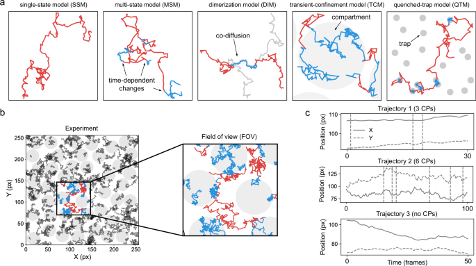
a Examples of 2-dimensional trajectories undergoing interactions inducing changes in their motion. From left to right: single-state model (SSM) without changes of diffusion; multi-state model (MSM) with time-dependent changes between different diffusive states (red and blue); dimerization model (DIM) where a particle (red) selectively interacts with another particle (gray) and the two transiently co-diffuse with a different motion (blue trajectory); transient-confinement model (TCM) where a particle diffuses inside (blue) and outside (red) compartments with osmotic boundaries (gray area); quenched-trap model (QTM) where a particle is transiently immobilized (blue) at specific loci through interactions with static features of the environment (gray areas). b An experiment (left panel) consists of simulations performed according to one of the models of interactions described in (a) (here showing a TCM experiment), with a set of parameters describing the dynamic interplay of the particles and/or the environment. From the same experiment, several fields of view (FOVs) are selected. Particles within the same FOV (right panel) diffuse and undergo interactions among themselves and/or with the environment (gray areas) that affect their trajectories. c Time traces of the coordinates of exemplary trajectories from the experiment depicted in (b), displaying changes of diffusion properties at specific times (changepoints CPs, dashed vertical lines). For the Challenge, the motion analysis can be either performed directly from the video recording of the FOV (Video Track) or from detected trajectories linking the coordinates of individual particles at different times (Trajectory Track).
In the simulations, each dynamic state is characterized by a distribution of values for the parameters K and α. For each trajectory, the values of K and α for each state are randomly drawn from Gaussian distributions with bounds α ∈ (0, 2) and K ∈ [10−12, 106] pixel2/frameα. The interaction distance and the radius of confinement or trapping have constant values across each experiment. Simulations are provided in generalized units (i.e., pixels and frames) that can be rescaled to meaningful temporal and spatial scales.
A detailed description of the simulation procedure is presented in Extended Methods.
Competition design
To enable the assessment of the performance of previously established methods while fostering the development of new approaches and the participation from diverse disciplines, the challenge was organized along two tracks:
For each track, datasets were provided according to a hierarchical structure (Fig. 2b, c) that includes:
-
Experiment—A given biological scenario defined by a model of interactions and a set of parameters describing the dynamic interplay of the particles and the environment.
-
FOV—A region of the sample where the recording takes place. Particles within the same field of view (FOV) can undergo interactions among themselves and/or with the environment.
-
Video (Video Track only)—Videos corresponding to each FOV.
-
Trajectory (Trajectory Track only)—Trajectory corresponding to the motion of an individual particle.
For both tracks, all particles used in the simulations and located in the FOV are provided/visualized (i.e., full labeling conditions). The effect of blinking or photobleaching was not taken into account.
In each track, participants could compete in two different tasks, as typically done in the analysis of experimental data:
-
Ensemble Task—Ensemble-level predictions providing, for each experimental condition, the model used to simulate the experiment, the number of states, and the fraction of time spent in each state. For each identified state, participants had to determine the mean and standard deviation of the distribution of the generalized diffusion coefficients K, and the mean and standard deviation of the distribution of the anomalous diffusion exponent α corresponding to the underlying motion.
-
Single-trajectory Task—Trajectory-level predictions providing for each trajectory a list of M inner CPs delimiting M + 1 segments with different dynamic behavior. For each segment, participants had to identify the generalized diffusion coefficient K, the anomalous diffusion exponent α corresponding to the underlying motion, and an identifier of the kind of constraint imposed by the environment (0 = immobile, 1 = confined, 2 = free (unconstrained, 0.05 ≤ α α
For each task, several metrics were evaluated (see Scoring and evaluation). Participants were allowed to provide partial submissions, e.g., including predictions for a limited subset of experiments or for specific parameters. For ranking purposes of the Challenge, missing predictions were scored with the worst possible value of the corresponding metric.
Competition overview
The 2nd AnDi Challenge was held between December 1, 2023, and July 15, 2024, on the Codalab platform. It was divided into three phases, namely Development, Validation, and Challenge. The Development Phase (5 months) was intended for the participants to set up their methods, test them, and familiarize themselves with the datasets and the scoring platform. An unlabeled dataset was available, and the public leaderboard showed scores obtained on this dataset. An online workshop was held on February 22, 2024, to instruct the participants about the details of the challenge. The Validation Phase (1 month) was a test of the actual final challenge. A new dataset (described in Challenge Dataset) was provided, and the leaderboard was again public. The Challenge Phase (15 days) was the final stage of the competition. A new dataset was provided, and the number of submissions per team was limited to 1 per day. The results were not publicly disclosed, and the leaderboard was made public only after the end of the competition. In total, we received 1343 submissions during the three phases. Participants registered in teams of 1 to 5 people. In the final stage, out of 80 registered participants, 53 individuals, divided into 18 teams, were included in the leaderboard (see Supplementary Table 2 for the list of participating teams). The teams’ affiliations spanned Europe (12 teams), Asia (6 teams), and America (1 team). From the final leaderboard, members of the top 5 teams in each task were invited to co-author this article. An overview of these teams and the methods is provided in Supplementary Information— Overview of Teams and Methods.
The results of the Challenge were discussed with the participants and other experts from the field during the 2nd Anomalous Diffusion Workshop that was held in June 2025.
Challenge dataset
The Challenge dataset was composed of 12 experiments corresponding to different diffusion models and parameter values. Details about the numeric values of parameters of the experiments are given in Supplementary Table 3. In addition, Supplementary Fig. 1 summarizes the distribution of specific features within the dataset. EXP 1 aimed at mimicking multistate diffusion in membrane proteins. Average diffusion coefficients and the transition matrix of the MSM were chosen to reproduce, with the appropriate scaling, the three fastest states reported for the diffusion of the α2A-adrenergic receptor80. EXP 2 reproduced changes in diffusion coefficient due to protein dimerization, inspired by the behavior reported for the epidermal growth factor receptor ErbB177. EXP 3, EXP 4, and EXP 5 were designed to compare the methods’ ability to detect changes from the same free diffusive state to a slow diffusing state characterized either by traps (QTM, EXP 3), small confinement regions (TCM, EXP 4), or a subdiffusive dimeric state (DIM, EXP 5). EXP 6 and EXP 7 were meant to assess the methods’ ability to take advantage of the knowledge of the physical model itself and additional information present in the experiment to improve predictions. The experiments corresponded to different theoretical models (DIM and MSM) with the same diffusive parameters. EXP 8 served as a negative control and contained only SSM trajectories with very broad distributions of K and α. EXP 9 was generated from QTM with very short trapping times and superdiffusion in the free state to assess how the methods deal with such extreme conditions. The other three experiments contained data with extreme and unrealistic parameters meant to assess potential biases of the methods, and will not be discussed further.
Scoring and evaluation
The performance of the methods was evaluated using specific metrics for each task. For ranking purposes in the Challenge, composite metrics were used, as described below.
Ensemble task
Participation in the Ensemble Task required predictions of the type of model used for simulating each experiment, the number of states S of the model, and the parameters of each state. The type of model was simply evaluated as correct or wrong. The prediction of the number of states was assessed by measuring the difference with the ground truth. For both the generalized diffusion coefficient and the anomalous diffusion exponent, predictions had to include the mean, the standard deviation, and the relative weight of each state. From these values, we computed the associated multi-modal distributions Pα and PD. The similarity of these distributions to the ground-truth distributions Qα and QD was assessed by means of the first Wasserstein distance (W1),
$${W}_{1}(P,Q)={\int}_{{\rm{supp}}(Q)}| {{\rm{CDF}}}_{P}(x)-{{\rm{CDF}}}_{Q}(x)| dx$$
(3)
where CDFQ is the cumulative distribution function of the distribution Q and supp(Q) is the support (α ∈ (0, 2) and K ∈ [10−12, 106] pixel2/frameα).
Single-trajectory task
Participation in the Single-trajectory Task required predictions of the M CPs and the dynamic properties, i.e., the generalized diffusion coefficient K, the anomalous exponent α, and diffusive-type identifiers of the resulting M + 1 segments. Different metrics were used to evaluate the methods’ performance.
CP detection metrics
Following Ref. 51, given a ground-truth CP at locations t(GT),i, and a predicted CP at locations t(P),j, we defined the gated absolute distance:
$${d}_{i,j}=\min (| {t}_{({\rm{GT}}),i}-{t}_{({\rm{P}}),j}|,{\varepsilon }_{{\rm{CP}}}),$$
(4)
where εCP was used as a fixed maximum penalty for CPs located more than εCP apart. For a set of MGT ground-truth CPs and MP predicted CPs, we solved a rectangular assignment problem using the Hungarian algorithm85 by minimizing the sum of distances between paired CPs:
$${d}_{{\rm{CP}}}=\mathop{\min }\limits_{{\rm{paired}}\,{\rm{CP}}}\left(\sum {d}_{i,j}\right).$$
(5)
The distance dCP allows to define a pairing metric:
$${\alpha }_{{\rm{CP}}}=1-\frac{{d}_{{\rm{CP}}}}{{d}_{{\rm{CP}}}^{\max }},$$
(6)
where \({d}_{{\rm{CP}}}^{\max }={M}_{{\rm{GT}}}\,{\varepsilon }_{{\rm{CP}}}\) is the distance associated with having all predicted CPs unpaired or at a distance larger than εCP from all ground-truth CPs. The metric αCP is bound in [0, 1], taking a value of 1 if all ground-truth and predicted CPs are matching exactly. Similarly, we define a CP localization metric:
$${\beta }_{{\rm{CP}}}=\frac{{d}_{{\rm{CP}}}^{\max }-{d}_{{\rm{CP}}}}{{d}_{{\rm{CP}}}^{\max }+\overline{{d}_{{\rm{CP}}}}},$$
(7)
where \(\overline{{d}_{{\rm{CP}}}}\) is the distance associated with having all unassigned predicted CPs at a distance larger than εCP from all ground-truth CPs. This metric measures the presence of spurious CPs and is bound in [0, αCP], taking value αCP if no spurious CPs are present. We also calculate the number of true positives (TP), i.e., the paired true and predicted CPs with a distance smaller than εCP. Spurious predictions, i.e., not associated with any ground truth or having a distance larger than εCP were counted as false positives (FP). Ground truth CPs not having an associated prediction at a distance shorter than εCP were considered false negatives (FN). Given an experiment containing N trajectories, we computed the overall number of TP, FP, and FN. We then used these values to calculate the JSC over the whole experiment as:
$${\rm{JSC}}=\frac{{\rm{TP}}}{{\rm{TP}}+{\rm{FN}}+{\rm{FP}}}.$$
(8)
For the predicted CPs classified as TP, we also computed the root mean square error (RMSE), defined as:
$${\rm{RMSE}}=\sqrt{\frac{1}{N}\sum _{\begin{array}{c}{\rm{paired}}\,{\rm{CP}}\\ {d}_{i,j}
(9)
Metrics for the estimation of dynamic properties
For the evaluation of the methods’ performances on the estimation of the dynamic properties, we first followed a procedure similar to the one described above for the pairing of the CPs. Predicted CPs were used to define the predicted trajectory segments. We defined a distance between predicted and ground-truth segments based on the JSC calculated with respect to their temporal support, where time points at which predicted and ground-truth segments overlap were considered as TP, predicted time points not corresponding to the ground truth as FP, and ground-truth time points not predicted as FN. The Hungarian algorithm was used to pair segments by maximizing the sum of the JSC. Only paired segments were used to calculate metrics assessing methods’ performance for the estimation of dynamic properties. For the generalized diffusion coefficient K, we used the mean squared logarithmic error (MSLE) defined as:
$${\rm{MSLE}}=\frac{1}{N}\sum _{\begin{array}{c}{\rm{paired}} \\ {\rm{segments}}\end{array}}{\left(\log ({K}_{({\rm{GT}}),i}+1)-\log ({K}_{({\rm{P}}),j}+1)\right)}^{2}.$$
(10)
For the anomalous diffusion exponents α, we used the mean absolute error (MAE):
$${{\rm{MAE}}}_{\alpha }=\frac{1}{N}\sum _{\begin{array}{c}{\rm{paired}}\\ {\rm{segments}}\end{array}}| {\alpha }_{({\rm{GT}}),i}-{\alpha }_{({\rm{P}}),j}|,$$
(11)
where N is the total number of paired segments in the experiment, α(GT),i and α(P),j represent the ground-truth and predicted values of the anomalous exponent of paired segments, respectively. For the classification of the type of diffusion, we used the F1-score:
$${{\rm{F}}}_{1}=\frac{2{{\rm{TP}}}_{{\rm{c}}}}{2{{\rm{TP}}}_{{\rm{c}}}+{{\rm{FP}}}_{{\rm{c}}}+{{\rm{FN}}}_{{\rm{c}}}},$$
(12)
where TPc, FPc, and FNc represent true positives, false positives, and false negatives with respect to segment classification. The metric was calculated as a micro-average, which aggregates the contributions of all classes to compute the average metric and is generally preferable when class imbalance is present.
Metrics for challenge ranking
For ranking purposes, we used the mean reciprocal rank (MRR) as a summary statistic for the overall evaluation of software performance42:
$${\rm{MRR}}=\frac{1}{N}\cdot \mathop{\sum }\limits_{i=1}^{N}\frac{1}{{{\rm{rank}}}_{{{\rm{M}}}_{{\rm{i}}}}},$$
(13)
where \({{\rm{rank}}}_{{{\rm{M}}}_{{\rm{i}}}}\) corresponds to the position in an ordered list based on the value of the corresponding metrics Mi.
For the Ensemble Task, the metrics involved in the calculation were the F1-score of the model and the MAE of the distributions of K and α. For the Single-trajectory Task, we used the JSC and the RMSE of CPs, the MSLE of K, and the MAE of α.
Overview of the challenge results
The Challenge dataset was comprehensively designed to test the submitted methods under distinct scenarios, using ad hoc metrics to evaluate their specific capabilities. For ranking, we employed composite metrics that aggregate the scores from different experiments and subtasks. The results are summarized in Fig. 3. Here, we present an overview of the Challenge results, highlighting the general trends observed. The complete rankings are provided in Supplementary Fig. 2.
Fig. 3: Challenge rankings.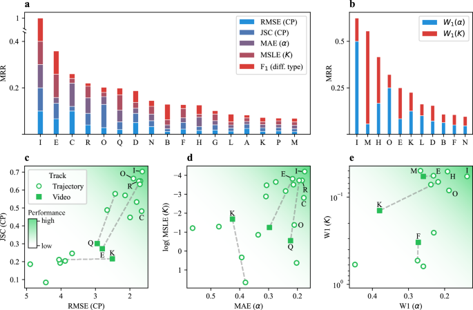
Mean reciprocal rank (MRR) of all methods participating in the Single-trajectory Task (a) and Ensemble Task (b) in the Trajectory Track. The colors represent the relative contributions of the metrics of each subtask to the overall MRR. c–e Correlation between subtask metrics associated with changepoint (CP) detection (c), the prediction of segment properties (d) in the Single-trajectory Task, and the prediction of diffusive properties in the Ensemble Task (e). Empty circles and filled squares represent the metrics obtained for the Video Track and the Trajectory Track, respectively. Dashed lines join results obtained by the same team in the two tracks. The darker background color indicates the area of the plot corresponding to better performances. Source data are provided as a Source Data file.
In the Single-trajectory Task (Fig. 3a), one method based on UNet3+86,87 (team I) clearly outperformed the others, whereas the Ensemble Task (Fig. 3b) showed a more balanced competition. From the MRR breakdown, we observed that the top team in the Single-trajectory Task performed consistently well across all metrics. In contrast, for the Ensemble Task, the top teams improved their final ranks by specializing in one of the two subtasks.
We also show the correlation between pairs of metrics associated with CP detection (Fig. 3c) and the prediction of diffusive properties (Fig. 3d, e). The predictions for the Video Track (represented by filled squares) are also included alongside those of the Trajectory Track (represented by empty circles). Across methods, enhanced CP detection, reflected by higher JSC and lower RMSE, yields a tight correlation between these metrics (Fig. 3c). A similar but weaker trend appears for K and α errors (Fig. 3d, e), because their estimation often relies on distinct algorithms, decoupling improvements in one from the other.
In the plots, the dashed lines connect the predictions of teams participating in both tracks. All teams in the Video Track (teams E and Q for the Single-trajectory Task, teams E and F for the Ensemble Task), except for team K, improved their predictions in the Trajectory Track compared to the Video Track. Notably, all four teams first extracted the trajectories using a previously established tracking method5,40,88,89,90,91 and then performed the ensuing analysis using the same method developed for the Trajectory Track. While this highlights the influence of error associated with the tracking process51, none of the methods explored the possibility of obtaining results directly from the video, which was one of the exploratory goals of this competition.
Finally, Fig. 4 shows the score obtained for subtask metrics by all teams for each experiment (filled symbols). The consistently lower performance of the Video Track compared to the Trajectory Track lends support to the third rationale: it suggests that challenges in accurately extracting trajectories from experimental videos represent a more significant bottleneck than the downstream analysis of pre-extracted tracks.
Fig. 4: Overview of the results.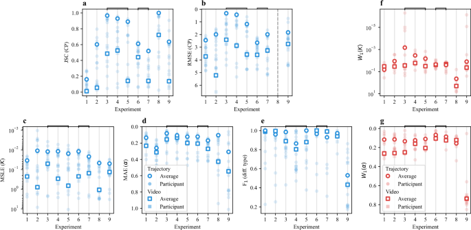
a–e Scores obtained for each subtask metric by all teams for each experiment of the Single-trajectory Task (filled symbols). Squares and circles represent the metrics obtained for the Video Track and the Trajectory Track, respectively. f, g Scores obtained for each subtask metric by all teams for each experiment of the Ensemble Task (filled symbols). Squares and circles represent the metrics obtained for the Video Track and the Trajectory Track, respectively. In all panels, open symbols represent average scores. The vertical axes are arranged so that the best performance is always shown at the top. Horizontal square brackets indicate groups of experiments that are discussed comparatively. Source data are provided as a Source Data file.
These plots provide further insight into which experimental conditions were more challenging for each subtask. For example, CP detection in EXP 1 (MSM with 3 states) was particularly difficult, as indicated by the low JSC in Fig. 4a. As shown in Fig. 4e, classification of the type of diffusion for EXP 4 (TCM) was more challenging than EXP 3 (QTM), despite having similar parameters for the unrestrained motion. For the Ensemble Task, we observe poorer predictions for K in EXP 8 (SSM, Fig. 4f) and for α in EXP 9 (QTM, Fig. 4g). In the following, we will comparatively discuss results obtained for groups of experiments aimed at detecting specific method capabilities. For most of these analyzes, we will mainly consider the methods of the top 5 teams in each Track and Task.
CP detection and segment diffusion properties
A main aspect of the Challenge was the evaluation of CP detection capability and the ensuing assessment of diffusion properties for the identified segments. In particular, we tested the methods’ ability to distinguish true anomalous diffusion from subdiffusive behavior that emerges solely from physical constraints, directly addressing the second rationale. These insights were provided by the Single-trajectory Task.
As shown in Fig. 4a–e, the methods generally performed well when tested on time-varying processes. We sought to characterize the false positive rate of the methods by evaluating their behavior over the trajectories of EXP 8 having no CPs (Fig. 5a, b). EXP 8 also served to assess the methods’ ability to estimate parameters K and α independently of errors induced by incorrect segmentations. Submitted predictions were benchmarked with the estimations of K and α obtained by linear and logarithmic fits of the MSD, respectively (dashed lines). Most methods predicted very few CPs for these trajectories, producing a low false positive rate and outperformed the MSD fit for both K and α (Fig. 5a, b).
Fig. 5: CP detection and segment diffusion properties.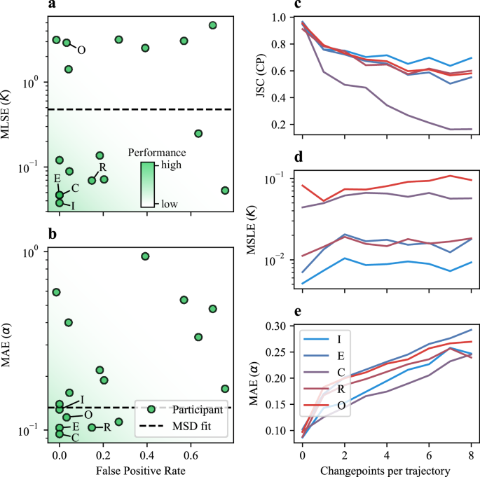
a, b Scatter plots of the metrics associated with segment diffusion properties in the Single-trajectory Task of the Trajectory Track as a function of the false positive rate calculated for EXP 8, composed of trajectories without CPs. Results obtained by all participants are shown. Dashed lines correspond to the scores obtained by using the fit of the mean-squared displacement, as a benchmark. The darker background color indicates the area of the plot corresponding to better performances. c–e Dependence of the JSC, MSLE, and MAE on the number of changepoints for the Single-trajectory Task of the Trajectory Track. Only the results of the top 5 teams are shown. The color code represents their position in the ranking (blue is the highest, red the lowest). Source data are provided as a Source Data file.
A relevant aspect associated with CP detection accuracy is its dependence on the number of CPs per trajectory, shown in Fig. 5c–e, which is inversely related to the average segment duration. As expected, the JSC shows worse performance as the number of CPs increases (Fig. 5c). Regarding the diffusion parameter estimation, we observe that the methods allow a robust estimation of K independently of the number of CPs (Fig. 5d), whereas for α we observe a drop in performance as the number of CPs increases (Fig. 5e). This confirms the difficulty of estimating α from short segments, due to its asymptotic nature, already observed in the 1st AnDi Challenge42.
Classification of types of diffusion
One of the goals of this competition was to assess the methods’ ability to classify different diffusion types and distinguish among distinct physical models. Results for all experiments of the Video and Trajectory Tracks are shown in Supplementary Figs. 3 and 4, respectively. The results of the two tracks were qualitatively similar but the Video Track had overall lower scores since all teams except team Q missed the immobile state (Supplementary Fig. 3). To summarize the methods’ ability to assign segments to diffusion types, in Fig. 6 we show the distribution of each diffusive state compared to the ground truth (horizontal segments) for representative experiments of the Trajectory Track. In Fig. 6a we exemplarily show the results obtained for EXP 9, a QTM with an unconstrained state having a narrow distribution of K but with α values that could produce either superdiffusive or directed motion. In this case, only the top method (team I, light blue) was able to produce a reliable classification of the diffusion type of the segments. The difficulty in inferring the correct type of mechanism producing interaction underscores the challenges in accurately analyzing this kind of data, which can have significant implications for the biological interpretation of the results. Although perfect classification of diffusive states remains challenging, the algorithms nonetheless provide precise estimates of critical biophysical parameters, namely, the average dwell times in both trapped and unconstrained states (inset of Fig. 6a). The measure of these parameters is essential for quantifying binding kinetics, confinement lifetimes, and transition rates that directly inform biological interpretation.
Fig. 6: Classification of types of diffusion.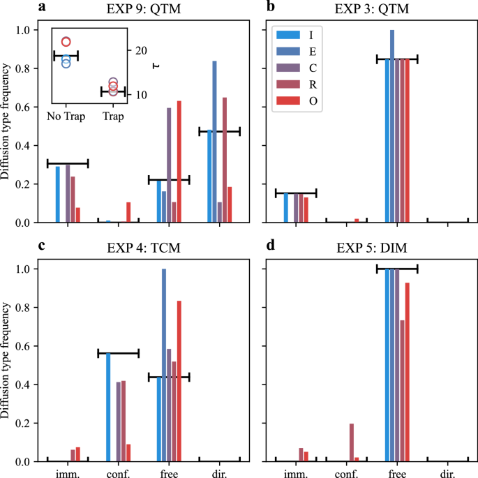
Only the results of the top 5 teams are shown; the color code represents their position in the ranking (blue is the highest, red the lowest). Predictions for the frequency of time spent with a given diffusion type for EXP 9 (a), EXP 3 (b), EXP 4 (c), and EXP 5 (d) for the Single-trajectory Task of the Trajectory Track. Horizontal segments represent the ground truth. Inset of (a) predicted average residence time for the trapped and non-trapped states. The non-trapped state includes segments corresponding to both unconstrained (free/anomalous) diffusion and directed motion. Source data are provided as a Source Data file.
The second rationale for the Challenge was to probe the methods’ ability to disentangle genuine anomalous diffusion from subdiffusive behaviors arising purely from motion constraints. To test the methods in challenging conditions, we designed a group of experiments (EXP 3, EXP 4, and EXP 5) with different underlying models but with diffusive parameters that produce similar trajectories. The three experiments share an unconstrained state with normal diffusion, and K ≈ 1: EXP 3 is simulated as QTM, whereas EXP 4 is from a TCM with a small confinement radius and α ≈ 0.2, and EXP 5 is DIM with a dimeric state with α ≈ 0.2. Other parameters were set to obtain similar residence times in the different states. Figure 6b–d highlights the performance of the top five methods across EXP 3–5. Teams I, C, and R each correctly classify over 95% of segments, closely matching the true distribution of diffusive states. Team E tends to over-label segments as diffusive, while Team O occasionally confuses confined segments for diffusive ones and vice versa. Team R, despite its high overall accuracy, also makes occasional misclassifications of diffusive segments as immobile or confined. Importantly, for EXP 4 (small-radius confinement) and EXP 5 (dimerization-induced subdiffusion), misclassification as immobile is negligible for Teams I, C, and R. Detecting confinement in EXP 4 is particularly challenging since short dwell times in confined areas yield few boundary reflections, inducing confusion with unconstrained anti-persistent subdiffusion of EXP 5. The ability of Teams I, C, and R to resolve these subtle cases underscores the high sensitivity and robustness of their methods.
Using physical models to enhance method performance
The information contained in an individual trajectory is typically sufficient to estimate CPs and diffusive properties. However, for some physical models, the knowledge of the model itself offers additional information that could be used to improve further CP detection and parameter estimation. This is the case for QTM and TCM, where changes in diffusion correspond to spatial constraints. For DIM, diffusion changes are associated with particle proximity; in addition, since particles in a dimer co-diffuse, one could, in principle, use twice as much information to estimate K and α, although in typical experimental conditions it may be very challenging to track two co-diffusing particles.
Along these lines, for the Single-Trajectory Task, the lowest JSC values were obtained for EXP 1 and EXP 7 (circles in Fig. 4a). Both experiments correspond to simulations of MSM, a model where the diffusion changes are produced in a purely time-dependent fashion and the dataset itself does not provide additional hints to determine them. This suggests that the methods can directly or indirectly take advantage of the presence of a physical event (e.g., trapping, confinement, or dimerization) to enhance CP detection accuracy. To assess this effect quantitatively, we used EXP 5 and EXP 6, which correspond to different physical models (DIM and MSM, respectively) generated with an identical set of diffusive parameters. To quantify model-based gains, we computed the relative improvement
$$\Delta m(\%)=\frac{{m}_{{\rm{DIM}}}-{m}_{{\rm{MSM}}}}{{m}_{{\rm{MSM}}}}\times 100\%$$
(14)
for each subtask metric (JSC, MSLE, and MAE). Figure 7 reports these improvements for all methods, with the overall average shown as a dashed line.
Fig. 7: Effect of the physical model.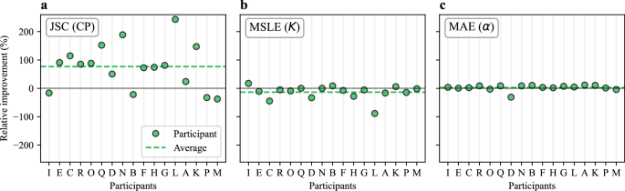
Relative improvement for all participants when predicting trajectory properties from EXP 5 (DIM) with respect to EXP 6 (MSM) for the Single-trajectory Task of the Trajectory Track. Each panel reports the metrics associated with a different subtask: JSC (a), MSLE (b), and MAE (c). Source data are provided as a Source Data file.
Surprisingly, while most of the methods showed improved performance for the CP prediction in DIM (Fig. 7a), there were minor differences in the prediction of diffusive properties (Fig. 7b, c). We believe this is because the methods predict each trajectory’s properties without considering it in the ensemble of the FOV or of the experiment, an observation that may improve the next generation of methods.
Ensemble predictions
The Ensemble Task was designed to test whether the methods could take advantage of the increased statistics obtained from common parameters shared by all trajectories within the same experiment to better identify the type of motion and estimate its parameters. As discussed earlier, several approaches of this type have been devised and used in the past to extract biophysical information from single-particle tracking data (Supplementary Table 1). However, no pure ensemble-level method, i.e., one that disregards the individual trajectory identity, was employed for the Challenge. Instead, all teams that provided submissions for the Ensemble Task used predictions obtained at the single-trajectory level, which were then pooled together to estimate the moments of the distributions of the diffusive parameters. Results for all experiments of the Video and Trajectory Tracks are shown in Supplementary Figs. 5–8. The resulting distributions are summarized in Fig. 8 for 4 exemplary experiments (EXP 4, EXP 7, EXP 8, and EXP 9) of the Trajectory Track. The pooling operation was performed using two general approaches: teams either applied a Gaussian mixture model (GMM) or a clustering algorithm on the predicted segments to extract subpopulation parameters, with four of the top 5 teams opting for the former approach (teams E, I, M, and O). Interestingly, as it can be inferred from Fig. 3a, b, the scores obtained by the teams participating in both tasks showed a low correlation. Therefore, accurate predictions at the single-trajectory level do not necessarily translate into reliable ensemble-level predictions, pointing to a critical role of the clustering approach.
Fig. 8: Ensemble task predictions for the trajectory track.
a–d show the predicted distributions of the diffusion coefficient K, and e–h the anomalous exponent α for EXP 4, EXP 7, EXP 8, and EXP 9, respectively. Distributions were computed from the estimated means and variances (see Scoring and evaluation—Ensemble Task). Only the results of the top five teams are displayed, with color indicating rank (blue is the highest, red the lowest). Black curves denote the ground-truth distributions. Source data are provided as a Source Data file.
Figure 8a, b shows an experiment where all teams provided consistent and reasonable predictions. This is particularly evident for the K distribution in EXP 7 and EXP 8 (Fig. 8b, c). Since the methods rely on estimates of K per segment and then apply GMM or k-means, they generally tend to over-fragment wide K ranges, misrepresenting the overall distribution. The corresponding predictions for the distributions of α for these experiments are shown in Fig. 8f, g. For EXP 8, characterized by the absence of CPs and nearly flat distributions of K and α, most methods successfully captured the broad distribution of α (Fig. 8g). However, their predictions for K (Fig. 8c) were often biased toward different ranges within the allowed support. In contrast, EXP 9 presented a population of short dwell times in the trapped state. Most methods successfully detected the occurrence of these events, as reflected in the K distribution (Fig. 8d), but, with the exception of team I, failed to associate these events with the correct α = 0 Fig. 8h.
We further point out that optimizing methods to provide high scores for the metrics of the competition did not always translate into more meaningful insights about the underlying physical processes. For instance, teams M, H, and O showed significant biases across all experiments when predicting the K distribution but still achieved high rankings according to the metric in Eq. (3) (Supplementary Fig. 6). Moreover, accurately predicting the number of true states did not provide a clear advantage with this metric, as most top teams overestimated the number of states but carefully adjusted their relative weights to minimize differences with the ground-truth distribution.
Results summary and take-home messagesRobust changepoint detection
Top single-trajectory methods (e.g., based on UNet3+86) consistently achieve over 95% accuracy in identifying segment boundaries, with only minor false-positive rates across all scenarios.
Distinguishing confinement, immobilization, and anomalous diffusion
Leading algorithms accurately classify segments arising from geometric constraints or anomalous dynamics. Only very short segments and exponents close to zero remain challenging, indicating minimal crosstalk between distinct diffusion mechanisms.
Trajectory extraction is a bottleneck
Video-Track performance lags the Trajectory Track by 10−30%, highlighting that linking and localization errors-not downstream analysis–drive most of the accuracy loss.
Parameter estimation benefits from physical priors
Incorporating known physical models may yield significant gains in changepoint detection, but separate estimation pipelines for K and α result in only modest improvements in parameter accuracy.
Dedicated ensemble approaches are needed
Ensemble Task submissions rely on GMM or k-means clustering of per-trajectory outputs, which fragments broad parameter distributions (e.g., EXP 7–8). Ensemble approaches, either bypassing single-trajectory clustering or using more sophisticated grouping techniques, hold potential for uncovering population-scale insights.