Experimental methods
The experiments were performed by combining a monochromatized table-top high-harmonic-generation (HHG) source, a liquid micro-jet and an electron-electron coincidence photoelectron spectrometer, as shown in Fig. 7(a). The extreme-ultraviolet (XUV) pulses were delivered by a time-preserving monochromator. High-harmonic generation was driven by a near-infrared laser pulse of ~1.2 mJ and ~30 fs duration centered at 800 nm with a repetition rate of 5 kHz. For the XUV energies below 60 eV, the driving pulse was focused into a semi-infinite gas cell filled with 25 mbar of neon, and the generated harmonics were collimated by a toroidal mirror (TM1) and spatially diffracted by a 300 lines/mm grating mounted in conical-diffraction geometry. For the generation of photon energies above 60 eV, instead of the semi-infinite gas cell, we used a 3 mm diameter metallic tube filled with 19 mbar of neon to extend the cut-off energy of the HHG spectrum. Accordingly, a higher groove density grating (600 lines/mm) was introduced to efficiently separate the generated harmonics. The diffracted harmonics were then focused by a second toroidal mirror (TM2) onto a 50 μm slit to select a single harmonic order. Finally, the XUV beam containing only a single harmonic order was imaged by a third toroidal mirror (TM3) onto the liquid micro-jet in the interaction chamber.
Fig. 7: Schematic illustration of the experimental setup.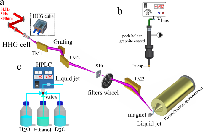
a Scheme of the XUV-monochromator, adapted from Fig. 1a in ref. 31. b Illustration of how the bias potential is applied to the liquid jet. c Illustration of the liquid system allowing for switching between liquid H2O and D2O under identical experimental conditions.
Liquid water was delivered into the chamber through a 25 μm inner-diameter quartz nozzle, which was capped with Cu tape, held together by Sn solder to prevent the insulating quartz from charging up due to stray electrons. The nozzle mounting system is made of PEEK and graphite-coated to ensure electrical conductivity (see Fig. 7(b)). The electrokinetic charging effect of the jet was minimized by adding NaCl at a concentration of 50 mmol/L. Moreover, a bias voltage of 0.45 V was applied to the liquid jet to simultaneously compensate the effects of the residual streaming potential and that of the vacuum-level offset between the jet and the photoelectron spectrometer35. A commercial HPLC pump from WATREX Prague (Model: P102) was utilized to transport the liquid sample into the chamber, the flow rate was set to 1.5 mL/min, while the stagnation pressure was maintained as 13.5 bar. In order to maintain identical experimental conditions, for each measurement at the same XUV energy, the liquid H2O and D2O were switched via a three-way valve immediately after one measurement was finished (see Fig. 7(c)).
The electrons emitted from the liquid jet were recorded by a magnetic-bottle photoelectron spectrometer, previously described in48, consisting of a permanent magnet (1 T), holding a conical iron tip, a 910 mm-long flight tube equipped with a solenoid that generates a homogeneous magnetic field of 1 mT along the flight tube. In this configuration, electrons with a pitch angle between 0° and ~120° are collected, corresponding to a solid angle of 2.8π sr. Without applying any bias potential on the skimmer and the flight tube, the spectrometer was first calibrated by photoionization of argon with various harmonics (H11–H51), the XUV energy was calibrated to an accuracy of ±0.06 eV. The average energy resolution of the spectrometer was estimated as ≈55:1 for the measured electrons in this study.
It is well known that the detection efficiency of a magnetic bottle spectrometer varies for photoelectron kinetic energy below ~1 eV49 and remains relatively constant for photoelectron kinetic energies between 1 and 100 eV50. Therefore, in order to enhance the detection efficiency of the slow electrons (
Theoretical methodsThe QM:QM fragmentation approach
Calculating the energies of molecules within large clusters presents significant challenges. Traditional quantum chemistry methods are often impractical due to their computational requirements or conceptual problems with highly excited states.
To address these challenges, we employed a stable and accurate fragmentation method that approximates the system by treating each molecule as an individual fragment51. For each fragment, we calculated the static point charges of its atoms. Once the charges were determined, a fragment was selected and surrounded by the point charges of the other fragments, representing the solvation effect. The energy of this fragment was then computed. This process was repeated for every fragment in the system, after which the total energy was obtained by summing the individual fragment energies. Note that the energy calculation for each fragment is influenced by the surrounding charges. Consequently, we can refine the point charges iteratively, leading to a self-consistent cycle that continues until the energy reaches a satisfactory level of precision. The final expression of the total energy, Etotal, is given as:
$${E}_{{{{\rm{total}}}}}={\sum}_{i=1}^{n}{E}_{i}-{\sum}_{A} {\sum}_{A
(2)
where i denotes the fragment index, Ei is the energy of the ith fragment, n is the total number of fragments, QA and QB are the charges of atoms A and B, and RAB is the distance between these two atoms. The second term in equation (2) subtracts the potential energies between atoms belonging to different fragments, thereby avoiding the double counting of these interactions.
This method defines two regions: one representing the solvent and the other representing the central molecule or cluster. Both regions can be treated using the same or different levels of theory. The fragmentation approach significantly reduces computational time while maintaining high accuracy, even for very large systems, without sacrificing the granularity of the solvent.
In this study, we focused on a pure water cluster, aiming at calculations of energies for two distinct states of the water dimer in the central reaction zone. The first state corresponds to the energy of the 2a1 inner-valence ionized state of the dimer, where the electron hole was generated using the Maximum Overlap Method (MOM)52. The second state corresponds to the energy of the doubly ionized dimer.
To construct the potential-energy curves, we elongated the OH bond of the initially ionized water molecule, which participates in proton transfer. This bond was stretched from ~1 Å to 2 Å, while the second OH bond of the same water molecule was elongated by half the distance of the first bond. During this process, only the hydrogen atoms were allowed to move, with the remaining atoms in the dimer held fixed. By plotting the total energy of the ionized dimer as a function of the OH bond length and subtracting the total energy of the ground state (with no bond elongation), we obtained the potential energy curves. The kinetic energy was then calculated as the difference between the potential energy curves of the doubly ionized state and the 2a1 ionized state. We also modeled the influence of cluster size on the behavior of these potential curves, treating the dimer as the core region and the solvent as a collection of additional water molecules.
The calculations were performed using Q-Chem 5.4 with the MP2 method, employing the aug-cc-pCVTZ basis set for oxygen and aug-cc-pVTZ for hydrogen53. We generated twenty different potential energy curves for various cluster sizes. However, convergence issues led to missing data points, complicating the computation of kinetic-energy values, which require matching points from both the 2a1 ionization and double-ionization states at the same OH bond length.
Initial geometries were sampled using quantum molecular dynamics simulations performed with our in-house software, ABIN version 1.154. The simulation temperature was set to 300 K and maintained using a Generalized Langevin Equation (GLE)44 thermostat. The time step was set to 40 atomic units, with a maximum of 100,000 steps. The first 10 ps of the simulation were treated as the thermalization phase, and twenty geometries were selected evenly from the remaining simulation time.
Modeling kinetic energy distributions and ICD efficiencies
To model the distribution of ICD-electron kinetic energies in large clusters, several key assumptions must be established. Our approach is to utilize geometries of the water dimer, as obtained from molecular simulations in a vacuum. In this context, we assume that the motion of the central dimer is largely independent of the cluster size. The geometry of the dimer evolves over time, described by its trajectory, which is characterized by two primary variables: time and the hydrogen-oxygen distance.
Initial conditions for these trajectories were generated using molecular dynamics simulations, performed with the ABIN54 code, while electronic energies were computed using the TeraChem software. The dynamical calculations were executed on the PBE/6-31++G⋆⋆ potential energy surface. The system’s temperature was controlled at 250 K using a GLE thermostat44. The time step was set to 20 atomic units (au), and the simulations were run for a maximum of 100,000 steps. The first 10 ps of the simulation were dedicated to thermalization, and from the remaining time, one hundred initial conditions were evenly sampled for further analysis.
The dynamics in the inner-valence ionized state was generated through classical molecular-dynamics simulations using the ABIN54 code, employing the MOM as implemented in the Q-Chem version 6.053. These simulations were performed in a microcanonical ensemble. The time step was set to 10 atomic units (au), with a maximum of 500 steps, though some trajectories were cut short due to convergence issues. Despite these challenges, we successfully obtained one hundred distinct trajectories for analysis.
To estimate the ICD-electron kinetic energy based on the dimer trajectories, we utilized potential energy curves derived from fragment-based methods. The kinetic energy was determined by the difference between the potential energy curves of the 2a1 state and the doubly ionized state. We generated twenty such potential energy curves, which were then fitted to a fourth-degree polynomial. Additionally, we fitted the standard deviation of the kinetic energy points using also a fourth-degree polynomial to account for variations.
In summary, while each trajectory exhibits unique characteristics, the overall kinetic energy function remains consistent for a given cluster size. Before implementing the Monte-Carlo algorithm, it is necessary to describe the energetic processes and corrections that influence the overall system behavior.
In the first assumption, we consider that the doubly-ionized state can decay into one of eleven possible states. The first state is the triplet ground state, while the next five are triplet excited states with energy shifts of 2.25, 2.3, 4.6, 6.0, and 8.0 eV, respectively, from the lowest to the highest energy levels. For simplicity, we assume these energy shifts remain constant, regardless of changes in the O-H bond distance. The remaining five states belong to the singlet manifold, with energies ~0.5 eV higher than their corresponding triplet states.
The second assumption introduces a time-dependent function to model the energy reduction of the singly-ionized state due to non-adiabatic interactions. This energy decrease is represented by a simple linear function, Edrop = δ ⋅ t, where t is time and δ is a constant that defines the rate of energy loss over time.
We can now construct the overall energy balance and corrections as described in equation (3). The kinetic energy, Ekinetic, is sampled from a normal distribution, where the mean value is determined by the fitted kinetic energy function, and the standard deviation is derived from the second fitted function. The term Estate accounts for the energy correction corresponding to the singlet or triplet states of the doubly-ionized species, while Edrop represents the systematic decrease in energy over time, governed by the constant δ.
To estimate the energy in the bulk phase, Ebulk is set to 2 eV, and we use the kinetic energies corresponding to the largest available cluster size of 216. If the bulk phase is not considered, Ebulk is set to zero.
$${E}_{{{{\rm{kinetic}}}}}={E}_{{{{\rm{distribution}}}}}-{E}_{{{{\rm{state}}}}}-{E}_{{{{\rm{drop}}}}}+{E}_{{{{\rm{bulk}}}}}$$
(3)
Next, we describe the algorithm. We start at time zero when the 2a1 electron-hole forms. From this point, we proceed in 0.24 fs time increments. At each step, we check whether the kinetic energy, Ekinetic, is positive. If the kinetic energy is positive, we randomly select one final state (if multiple states with positive Ekinetic exist). With a probability equal to \(\frac{\Delta t}{\tau }\), where τ is the parameter representing the ICD lifetime and Δt is the time step of 0.24 fs, ICD-electron emission occurs, and we record the kinetic energy. If no electron emission occurs, the trajectory continues to the next step. If the kinetic energy becomes negative, the trajectory may still proceed to a region where the ICD channel reopens, restoring positive kinetic energy and enabling electronic decay.
For better statistical accuracy, we run each trajectory one thousand times, resulting in a total of one hundred thousand potential ICD-electron emissions. This allows us to calculate the efficiency as the ratio between the number of emitted electrons and the maximum number of possible trajectories.
The dimer is the only system for which we can fully model the distribution of ICD electrons because it allows us to directly compute the kinetic energy at every point along each trajectory. For this purpose, we employed the QM approach with the same settings used for the potential energy curves. The algorithm is essentially the same as the one used in the Monte Carlo simulations above, but in this case, the kinetic energies are directly obtained from the QM calculations at each point along the trajectory. In this simulation, we did not account for the energy decrease of the singly-ionized state as all the trajectories become inactive very fast.
Reporting summary
Further information on research design is available in the Nature Portfolio Reporting Summary linked to this article.