Design and architecture of an arbitrary refractive function generator (RFG)
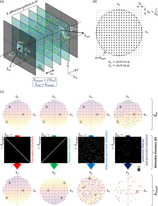
The architecture of an RFG is shown in Fig. 1a. A set of \(K\) optimized transmissive surfaces, placed between the input and output apertures, form the core of an RFG. For this work, we only consider phase-only surfaces that modulate the phase of the incident wave. Without loss of generalization, the amplitude modulation is assumed to be negligible, which is a valid assumption here, considering the short axial thickness of an RFG design. The RFG redirects a given input wave, propagating along the direction defined by the unit vector \({\hat{k}}_{{in}}\), into the output direction \({\hat{k}}_{{out}}\) such that \({\hat{k}}_{{out}}\approx {\hat{k}}_{{target}}\), where \({\hat{k}}_{{target}}=f({\hat{k}}_{{in}})\) and \(f\) is the target/desired refractive function, defining the mapping between the input and output directions. The unit vector \(\hat{k}\) denotes the direction of the wavevector \(\vec{k}\) of a plane wave, i.e., \(\vec{k}=\frac{2\pi }{\lambda }\hat{k}\), where \(\lambda\) is the wavelength of light. The unit vector \(\hat{k}\) encapsulates the two angles \(\theta\) and \(\varphi\), i.e., polar/zenith angle and azimuthal angle52 in a spherical coordinate system (see Fig. 1a), describing the propagation direction as follows:
$$\hat{k}=\left[\begin{array}{c}{k}_{x}\\ {k}_{y}\\ {k}_{z}\end{array}\right]=\left[\begin{array}{c}\sin \theta \cos \varphi \\ \sin \theta \sin \varphi \\ \cos \theta \end{array}\right]$$
(1)
Since \({k}_{z}^{2}=1-{k}_{x}^{2}-{k}_{y}^{2}\), a more succinct representation of \(\hat{k}\) is the 2D-vector \(({k}_{x},{k}_{y})\)53. Although \(\theta\) and \(\varphi\) can be continuous in principle, the resolution \({\delta }_{k}\) of \({k}_{x}\) and \({k}_{y}\) allowed by a finite aperture of dimension \({D}_{a}\) is also finite54, i.e., \({\delta }_{k}\approx \frac{\lambda }{{D}_{a}}\). Therefore, for a given acceptance angle \({\theta }_{\max }\) (the maximum angle with respect to the \(z\) axis), the set \({\mathbb{K}}\) of all \(\hat{k}\) vectors of interest can be written as: \({\mathbb{K}}{\mathbb{=}}\{({k}_{x},{k}_{y}):{k}_{x}=p\frac{\lambda }{{D}_{a}},{k}_{y}=q\frac{\lambda }{{D}_{a}},{k}_{x}^{2}+{k}_{y}^{2} where \(p\) and \(q\) are integers. The elements of this set are represented by the dots within the circle of radius \(\sin {\theta }_{\max }\) in Fig. 1b, and can be enumerated as \(\{{\hat{k}}_{1},{\hat{k}}_{2},\cdots,{\hat{k}}_{{N}_{m}}\}\) where \({N}_{m}=\left|{\mathbb{K}}\right|\) is the number of elements in \({\mathbb{K}}\). An arbitrary refractive function \(f\) can be thought of as a mapping from \({\mathbb{K}}\) to \({\mathbb{K}}\), i.e., \(f:{\mathbb{K}}{\mathbb{\to }}{\mathbb{K}}\). Each of the dots, defining the set \({\mathbb{K}}\), represents a ‘direction’ that the input or output wave can have.
The mapping of \({\mathbb{K}}\) under an arbitrary refractive function \(f\) can be described by a binary \({N}_{m}\times {N}_{m}\) matrix \(R\) (such as the ones shown in Fig. 1c), where the 1’s in the matrix define the coupling between \({\hat{k}}_{{in}}\) and \({\hat{k}}_{{target}}\). In other words, \(R[p,q]=1\) implies that if \({\hat{k}}_{{in}}={\hat{k}}_{q}\), then \({\hat{k}}_{{target}}=f({\hat{k}}_{{in}})={\hat{k}}_{p}\) where \(p,q\in \left\{{{\mathrm{1,2}}},\cdots,{N}_{m}\right\}\). We show a few examples of such matrices \(R\) and the corresponding mappings of the input directions in Fig. 1c, where each mapping is encoded in the color of the elements of \({\mathbb{K}}\). For example, an identity matrix (first column of Fig. 1c) represents the free-space refractive function (\({\hat{k}}_{{target}}={\hat{k}}_{{in}}\) or \({\theta }_{{target}}={\theta }_{{in}},{\varphi }_{{target}}={\varphi }_{{in}}\)), whereas the flipped identity matrix (second column of Fig. 1c) represents the negative refractive function (\({\theta }_{{target}}={\theta }_{{in}},{\varphi }_{{target}}={\varphi }_{{in}}+{180}^{\circ}\)). A more general form of an arbitrary refractive function can be represented by an arbitrarily selected permutation matrix, which defines an arbitrary mapping between \({\hat{k}}_{{in}}\) and \({\hat{k}}_{{target}}\) (third column of Fig. 1c). As another alternative for \(f\), we can also envision an arbitrarily filtered and permuted refractive function (fourth column of Fig. 1c), where the input waves traveling in certain arbitrarily chosen directions (the ones corresponding to the columns with all zeros) are filtered out, whereas the waves in the other directions are redirected in a manner following the permutation defined by \(f\) or the corresponding \(R\).
The design of an RFG follows supervised learning using pairs of input direction \({\hat{k}}_{{in}}\) (equivalently, \({\theta }_{{in}},{\varphi }_{{in}}\)) and target direction \({\hat{k}}_{{target}}\) (equivalently, \({\theta }_{{target}},{\varphi }_{{target}}\)), defined based on the desired/target refractive function \(f\) represented by \(R\). This involves angular spectrum-approach based numerical simulation of wave propagation through a digital model of the RFG (see the “Methods” section). For a wavefront corresponding to \({\hat{k}}_{{in}}\) at the input aperture, the wavefront leaving the output aperture is numerically simulated; the error between the output wavefront and the wavefront corresponding to \({\hat{k}}_{{target}}\) is backpropagated to update and iteratively optimize the surface phase features using a gradient descent-based algorithm; see the “Methods” section for details. Unless otherwise stated, we assumed an operating wavelength of λ = 0.75 \({{{\rm{mm}}}}\) for the results shown in the following sections. However, we emphasize that the presented conclusions hold for any wavelength of interest, as long as the dimensions are scaled proportionally to the illumination wavelength, \(\lambda\).
The results and analyses presented in the subsections leading up to the “Experimental results” as well as the animations presented in the Supplementary Movies 1–4 are based on numerical simulations. Unless otherwise stated, each diffractive surface in these simulations consists of \(200\times 200\) independently optimized phase features/elements. Each phase element spans an area of \(0.53\lambda \times 0.53\lambda\), resulting in a total surface width of \(106\lambda\). For arbitrary permutation refractive functions, both the input and output apertures have a width of \(10.6\lambda\); for negative refractive functions, this width is set to \(15.9\lambda\). The separation between consecutive planes—whether they contain input/output apertures or diffractive surfaces—is set to \(6\lambda\), unless specified otherwise. The maximum input polar angle \({\theta }_{\max }\) is assumed to be \({60}^\circ\).
Arbitrarily permuted refractive functions
We begin with the design of an arbitrarily permuted refractive function, where the target mapping between the input and output directions is defined by an arbitrarily chosen permutation matrix \(R\) (see Fig. 2a and the 3rd column of Fig. 1c). We designed an RFG comprising \(K=8\) structured surfaces to implement this refractive function, where the axial distance between two consecutive surfaces \({z}_{{ll}}\) was \(6\lambda\), giving an axial span of \({z}_{1K}\approx 50\lambda\) between the first and the last layers. The optimized phase profiles of these surfaces are shown in Fig. 2c. For each input direction \({\hat{k}}_{{in}}\), the corresponding output angle error is also shown in Fig. 2b. This output angle error \(\varepsilon\) is defined as the angle between \({\hat{k}}_{{out}}\) and \({\hat{k}}_{{target}}=f({\hat{k}}_{{in}})\). The estimation of the output wave direction \({\hat{k}}_{{out}}\) from the output wavefront is described in the “Method” section. Figure 2b reveals that the angular errors between the output directions and the target directions are negligible (less than \(0.1{4}^\circ\)), revealing the success of the RFG in implementing the arbitrarily permuted refractive function, i.e., \({{\hat{k}}_{{out}}\approx \hat{k}}_{{target}}=f({\hat{k}}_{{in}})\). Supplementary Movie 1 also shows the far-field output intensity as the input wave direction is swept, together with the corresponding target patterns that follow \(f\).
Fig. 2: Arbitrarily permuted refractive function implementation with a K = 8 RFG design.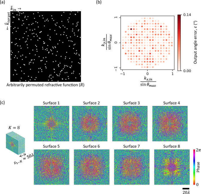
a The matrix \(R\) representing the arbitrarily permuted refractive function, the same as the one depicted in Fig. 1c, 3rd column. b The error in output angles for all the input directions. c The optimized phase profiles of the RFG surfaces. Here \({z}_{{ll}}\approx 6\lambda\), giving a total axial thickness of \({z}_{1-K}\approx 50\lambda\) between the first and the last surfaces.
In Fig. 3, we further analyze the errors of the refractive function implementation as the wavelength \({\lambda }_{{test}}\) of the input light deviates from the design wavelength \({\lambda }_{{train}}\) that the RFG is trained to operate at. While evaluating the error as a function of \({\lambda }_{{test}}\), we kept the input and target directions at \({\lambda }_{{test}}\) the same as those at \({\lambda }_{{train}}\). At each test wavelength \({\lambda }_{{test}}\), the distribution of the angular errors (over \({N}_{m}\) different input directions) is encapsulated with a box-and-whisker diagram in Fig. 3a. As expected, the error increases as \({\lambda }_{{test}}\) deviates from \({\lambda }_{{train}}\). However, the angular errors remain below \({4}^\circ\) over a wavelength range of \(\sim 0.99{\lambda }_{{train}}\) to \(\sim 1.01{\lambda }_{{train}}.\) The resilience against changes in wavelength can be improved by incorporating random wavelength variations during training. In Fig. 3b, we report the angular error of another design which was trained by randomly selecting the illumination wavelength from a desired range of interest during training, i.e., \({\lambda }_{{train}} \sim {{{\rm{Uniform}}}}\)(742.5 μm,757.5 μm). The angular errors of this “vaccinated” design remain limited to \(\sim \! {1}^\circ\) over the same wavelength range, showing the flexibility of our design approach to adapt to different requirements.
Fig. 3: Wavelength sensitivity and compactness of RFGs.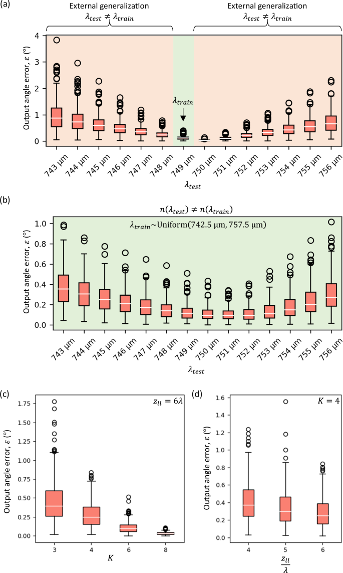
a Distribution of the output angle error as a function of the test wavelength \({\lambda }_{{test}}\), for the same RFG of Fig. 2, which was trained for an illumination wavelength of \(750\,{{{\rm{\mu }}}}{{{\rm{m}}}}\), i.e., \({\lambda }_{{train}}=750\,{{{\rm{\mu }}}}{{{\rm{m}}}}\). The distributions arise from the values corresponding to all the input directions. b Distribution of the output angle error as a function of the test wavelength \({\lambda }_{{test}}\), for an RFG design “vaccinated” against changes in wavelength. c Distribution of the output angle errors as a function of \(K\), while \({z}_{{ll}}\) is kept constant at \(\sim \! 6\lambda\). d Distribution of the output angle errors as a function of \({z}_{{ll}}\), while \(K\) is kept constant at \(4\).
Figure 3 further depicts the dependence of the output errors on the number of structured surfaces \(K\) and the surface-to-surface distance \({z}_{{ll}}\) comprising the RFG structure. For Fig. 3c, we decreased \(K\) from 8 to 3, keeping \({z}_{{ll}}=6\lambda\). The output angle errors increased as \(K\) decreased; however, we can see that the errors remain below \(1^\circ\) even when \(K\) is decreased to 4. For Fig. 3d, we set the number of structured surfaces \(K=4\) and reduced the surface-to-surface distance \({z}_{{ll}}\) from \(6\lambda\) to \(4\lambda\). On average, the output error increased with a decrease in \({z}_{{ll}}\). However, even with \(K=4\) and \({z}_{{ll}}=4\lambda\), the output angle errors stay below \(1.6^\circ\), demonstrating an arbitrarily permuted refractive function with an RFG spanning only \(\sim \! 15\lambda\) along the axial direction. To clarify, each \(K\) (\({z}_{{ll}}\)) value in Fig. 3c (3 d) represents a separately trained RFG design for the same target refractive function as in Fig. 2a.
An important metric of an RFG design is the output diffraction efficiency (\({{{\rm{DE}}}}\)), i.e., ratio between the diffracted output power along the target direction and the incident power at the input aperture; see the “Methods” section. For the RFG reported in Fig. 2, the diffraction efficiencies along the target directions ranged from 0.07% to 0.62%, see the 1st row of Fig. 4a. We can tune the diffraction efficiency of an RFG design by properly modifying the training loss function. By using an additional term in the loss function, weighted by \(\eta\) (a training hyperparameter), which penalizes against low diffraction efficiency, we can improve the output diffraction efficiencies of the resulting design with a relatively small sacrifice in the output error performance. For example, by using \(\eta=30\), we can have an RFG design where the maximum output angle error is \(0.87^\circ\), while the minimum diffraction efficiency increases to 2.75% (see the 3rd row of Fig. 4a). Figure 4b further summarizes the trade-off between the RFG performance and the output diffraction efficiency as a function of \(\eta\).
Fig. 4: Enhancement of the output diffraction efficiency of an RFG designed for an arbitrarily permuted refractive function.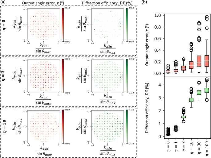
a Output angle errors and diffraction efficiencies of three different RFG designs trained with different values of the hyperparameter \(\eta\) (see Eq. (12)). Here, the target refractive function is the one shown in Fig. 2a. b Distribution of output angle errors and diffraction efficiencies as a function of \(\eta\). Each value of the training hyperparameter \(\eta\) corresponds to a separately optimized RFG design. For all the designs, \(K=8\) and \({z}_{{ll}}\approx 6\lambda\).
Arbitrarily filtered and permuted refractive functions
Next, we demonstrate the case of an arbitrarily filtered and permuted refractive function. Figure 5a depicts the target refractive function in this case. Here, ~90% of the input directions are filtered out at the output aperture, whereas the rest are redirected as specified by the non-zero elements of \(R\); stated differently, \(R\) in this case refers to an arbitrary permutation matrix with ~90% of its columns replaced with zeros, corresponding to the filtering of specific directions of input light. To implement this filtered refractive function, we designed an RFG comprising \(K=8\) surfaces, where the distance between consecutive surfaces \({z}_{{ll}}\) was \(6\lambda\), yielding an axial span of \({z}_{1K}\approx 50\lambda\) between the first and the last surfaces. The optimized phase profiles of these surfaces are shown in Fig. 5e. Figure 5b reveals negligible errors in the output angles for the input directions which are not filtered. At the same time, the diffraction efficiencies along the targeted output directions are \( > 10\%\); see Fig. 5c. To evaluate the filtering operation, we also calculated the relative percentage of residual power (i.e., the ratio between the power at the output and the power at the input aperture; see the “Methods” section) for each one of the filtered out directions. As shown in Fig. 5d, the relative power transmission is
Fig. 5: Arbitrarily filtered and permuted refractive function implementation with a K = 8 RFG design.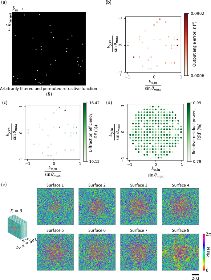
a The matrix \(R\) representing an arbitrarily filtered and permuted refractive function. The ratio of the filtered directions is ~90%. b Output angle error \(\varepsilon\) for all the unfiltered input directions. c Output diffraction efficiency \({{{\rm{DE}}}}\) for all the unfiltered input directions. d Relative residual power \({{{\rm{RRP}}}}\) for the filtered input directions. e The optimized phase profiles of the RFG surfaces.
Negative refractive function
We also considered a specific form of refractive function, i.e., the negative refractive function, where \({\theta }_{{target}}={\theta }_{{in}}\) and \({\varphi }_{{target}}={\varphi }_{{in}}+{180}^\circ\); see the third column of Figs. 1c and 6. To train for this refractive function, \({\theta }_{{in}}\) and \({\varphi }_{{in}}\) are randomly sampled from the uniform distributions \({{{\rm{Uniform}}}}\left({0}^\circ,{\theta }_{\max }={60}^\circ \right)\) and \({{{\rm{Uniform}}}}\left({0}^\circ,{360}^\circ \right)\), respectively. We designed an RFG comprising \(K=5\) surfaces for implementing the negative refractive function, and the optimized phase profiles are shown in Fig. 6c. For a dense grid of input directions \({\hat{k}}_{{in}}\), we show the corresponding output angle errors in Fig. 6a and the resulting diffraction efficiencies in Fig. 6b. While the maximum output angle error is \(\sim \! {2}^\circ\), this relatively large error occurs only when \({\theta }_{{in}}\) is close to \({\theta }_{\max }={60}^\circ\) because of the limited amount of training examples around these angular values at the edges. Figure 6d depicts the “operating curve” of this RFG, which plots the maximum acceptable input angle \({\theta }_{M}\) vs. the maximum acceptable output angle error \({\varepsilon }_{M}\), such that \(\varepsilon \le {\varepsilon }_{M}\) if \({\theta }_{{in}}\le {\theta }_{M}\). This plot shows that the RFG can operate at larger input angles if relatively larger errors are tolerated. For example, when \({\theta }_{{in}}\le 58^\circ,\) the output angle error stays below \(1^\circ\), as shown in Fig. 6e. Also, Fig. 6b plots the output diffraction efficiency for all the input directions, revealing high diffraction efficiency even without the use of a diffraction efficiency-related term in the training loss function.
Fig. 6: Negative refractive function (θtarget = θin, φtarget = φin + 180° for all θin θmax = 60°) using a K = 5 RFG design.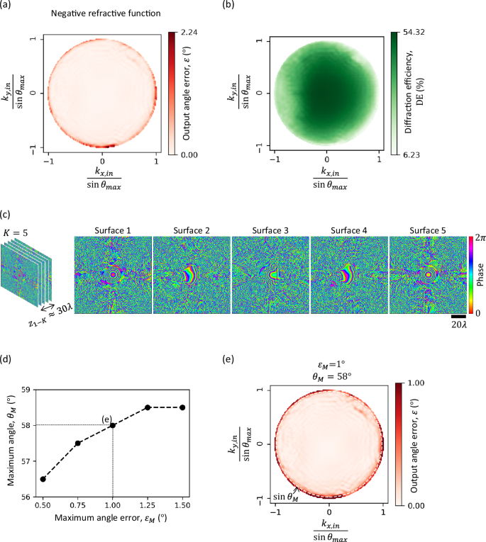
a Output angle error for all the input directions, sampled densely. b Diffraction efficiency for all the input directions. c The optimized phase profiles of the RFG surfaces. The distance \({z}_{{ll}}\) between consecutive surfaces is \(\sim 6\lambda\), giving an axial distance of \({z}_{1-K}\approx 30\lambda\) between the first and the last transmissive surfaces. d The operating curve of the RFG design, showing \({\theta }_{M}\) (the maximum acceptable \({\theta }_{{in}}\)) as a function of the maximum acceptable angle error, \({\varepsilon }_{M}\). e When \({\varepsilon }_{M}={1}^\circ\), \({\theta }_{M}={58}^\circ\), i.e., for all the input directions with \({\theta }_{{in}} , the output angle error is less than \(1^\circ\).
Wavelength multiplexing of arbitrarily permuted refractive functions
Wavelength multiplexing can be used to implement completely different refractive functions, simultaneously executed through the same RFG with a unique refractive function assigned to each wavelength of interest. We demonstrated this wavelength multiplexing capability by designing an RFG that performs three different arbitrarily permuted refractive functions at three different wavelengths, as shown in Fig. 7a, top row. Without loss in generality, we chose the refractive functions such that the corresponding permutation matrices \({R}_{1}\), R2, and \({R}_{3}\) do not have overlapping entries, i.e., \({\sum}_{m,n}{R}_{i}\left[m,n\right]{R}_{j}\left[m,n\right]=0\) if \(i \, \ne \, j\). We chose the wavelengths \({\lambda }_{1}=0.70\,{{{\rm{mm}}}}\), \({\lambda }_{2}=0.75\,{{{\rm{mm}}}}\), and \({\lambda }_{3}=0.80\,{{{\rm{mm}}}}\) to implement these refractive functions with an RFG comprising \(K=8\) surfaces. The refractive indices of the assumed RFG material at these wavelengths (\({\lambda }_{1},\,{\lambda }_{2},\,{\lambda }_{3}\)) are n1 = 1.6512, n2 = 1.6518, and n3 = 1.6524, respectively. The optimized thicknesses of the RFG surfaces are shown in Fig. 7b. As depicted in Fig. 7a (second row), the output angle error stays below \({0.5}^\circ\) for all the input directions for the three unique refractive functions at the three wavelengths, demonstrating the success of wavelength multiplexing of refractive functions performed simultaneously through the same RFG. Note from the second row of Fig. 7a that the set of input directions for these refractive functions are not identical, since the grid-spacing depends on the wavelength (see Fig. 1b).
Fig. 7: Wavelength multiplexing of arbitrarily permuted refractive functions with an RFG.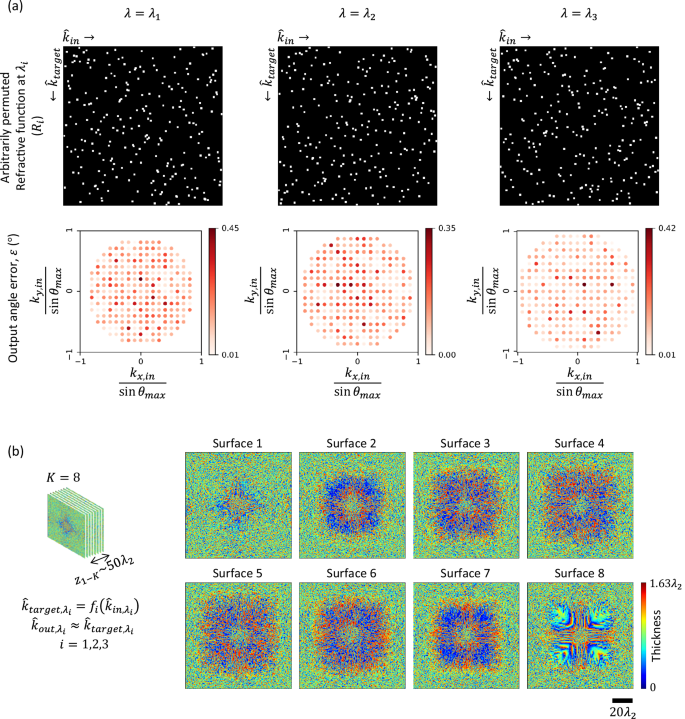
a The matrices representing the targeted arbitrarily permuted refractive functions at three distinct wavelengths (top row). The bottom row shows, for a \(K=8\) RFG design, the error in the output angle as a function of the input direction at these three wavelengths. b The optimized thickness profiles of the RFG surfaces. The distance \({z}_{{ll}}\) between consecutive surfaces is \(\sim 6{\lambda }_{2}\), giving an axial distance of \({z}_{1-K}\approx 50{\lambda }_{2}\) between the first and the last transmissive surfaces.
It is important to emphasize that this wavelength-multiplexed RFG design does not make use of the dispersion of the transmissive layers for its refractive function implementation accuracy; stated differently, even if we assume that the refractive indices of the assumed RFG material at these wavelengths (\({\lambda }_{1},\,{\lambda }_{2},\,{\lambda }_{3}\)) are equal, i.e., n1 = n2 = n3 = n, one could still perform wavelength-multiplexed refractive functions through an RFG design with the same level of accuracy and performance as shown earlier. Supplementary Fig. S2 compares the performance of an alternative design with flat dispersion, where n = 1.6518 was selected for all 3 wavelengths, revealing a statistically similar RFG performance as in Fig. 7. Supplementary Movie 2 also shows the far-field output intensity as the input wave direction is changed at these three wavelengths, together with the target patterns that follow the desired \({f}_{i}\) at the corresponding \({\lambda }_{i}\). These results indicate that the refractive function separation between different illumination wavelengths is based on the wavelength dependence of the free-space propagation kernel, and this unique capability does not need dispersion engineering of specialized materials, which is rather important for practical applications since one can readily work with almost any transmissive substrate that is available at a given desired spectral band.
Experimental results
We experimentally demonstrated the success of programmable refractive function implementation at THz part of the spectrum with an illumination wavelength of \(\lambda=0.75\,{{{\rm{mm}}}}\). We designed an RFG comprising \(K=3\) phase-only surfaces to implement the negative refractive function for \({\theta }_{{in}}\le {\theta }_{\max }\) \(={30}^\circ\). For this design, the width of the structured surfaces was selected as 80 mm, with a feature size of 0.4 mm, resulting in \(\sim\)0.12 million independently optimizable phase features for the RFG design. The distance between neighboring surfaces was \(\sim \! 16\lambda\), giving an axial span of \({z}_{1-K}\approx 32\lambda\) for the RFG design.
For resilience against potential misalignments during the experiment, the RFG design was “vaccinated” by applying random lateral shifts \(\left(\Delta x,\Delta y\right)\) to the surfaces during the digital training process. Similarly, the axial distances between the transmissive layers were also vaccinated against imperfections by adding random noise (\(\Delta z\)) in the optical forward model used during training. These random variables \(\Delta x\), \(\Delta y\), and \(\Delta z\) were sampled from uniform distributions, i.e., \({{{\rm{Uniform}}}}\left(-0.15\lambda,0.15\lambda \right)\). The optimized phase profiles of the resulting RFG surfaces are shown in Fig. 8a, together with the output angle errors and diffraction efficiencies obtained in numerical simulations.
Fig. 8: Experimental demonstration of the negative refractive function at λ = 0.75 mm.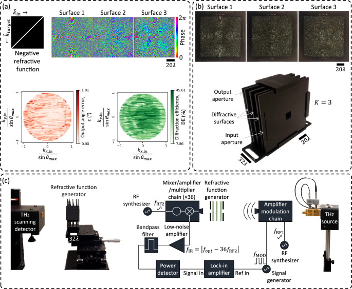
a The optimized phase profiles of a \(K=3\) RFG for implementing negative refractive function with \({\theta }_{\max }=30^\circ\). Also shown are the output angle errors and the diffraction efficiencies obtained in simulation. b The RFG hardware, assembled from the structured surfaces and input/output apertures, fabricated using 3D-printing. c The THz setup comprising the source and the detector, together with the 3D-printed RFG.
After the deep learning-based supervised design of the desired RFG, the optimized surfaces were fabricated using a 3D printer and assembled, together with the input and output apertures, to form the physical RFG, as shown in Fig. 8b. This physically assembled RFG was experimentally tested with the system shown in Fig. 8c, which comprises a THz source and a THz scanning detector; see the “Methods” section for details.
Figure 9 shows the experimentally measured output intensities at an axial distance of \(z=80\,{{{\rm{mm}}}}\) from the output aperture, together with the corresponding simulation results for different input wave directions defined by\(\,{\theta }_{{in}}\) and \({\varphi }_{{in}}\). During these experiments, the variation of \({\theta }_{{in}}\) was realized by moving the source horizontally along an arc (see Supplementary Fig. S1b), while the variation of \({\varphi }_{{in}}\) was implemented by in-plane rotation (relative to the source) of the RFG surfaces and the input and output apertures. To compensate for the relative rotation between the RFG and the detector plane, the fields of view (FOVs) corresponding to the experimental measurements were rotated by the same amount (in the opposite direction), as seen in Fig. 9. An additional calibration step to take into account the height of the source relative to the input aperture was also used; see Supplementary Fig. S1a.
Fig. 9: Visualization and quantitative analysis of the experimental RFG results.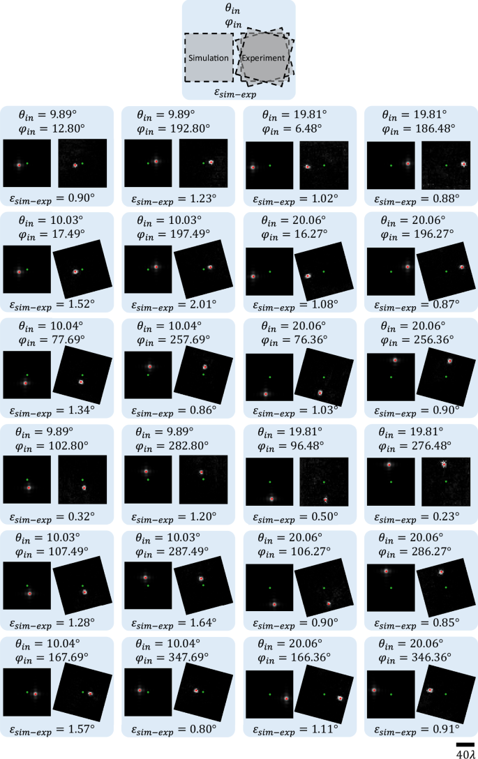
Each panel corresponds to the input direction defined by \(\left({\theta }_{{in}},{\varphi }_{{in}}\right)\) and compares the simulated and experimental diffraction patterns measured at a distance of \(z=80\,{{{\rm{mm}}}}\) from the output aperture of the RFG (see Fig. 9c). The green dot marks the center \(\left({{\mathrm{0,0}}}\right)\) of the FOV and the red dot marks the first moment of the diffracted intensity pattern; also see Supplementary Fig. S1b. In each panel, the mismatch between the numerical simulation and the experimental result, defined as the angle \({\varepsilon }_{{sim}-\exp }\) between the simulated output wave and the experimentally measured output wave, is also reported.
Visual assessment of the output intensity patterns in Fig. 9 reveals a very good agreement between the simulated patterns and the measured output patterns. For quantitative analysis, we estimated the direction of the output waves (\({\theta }_{{out}}\), \({\varphi }_{{out}}\)) from the first moments (center-of-mass) of the diffracted output intensity patterns, which are marked by red dots in Fig. 9; also see Supplementary Fig. S1b. To quantify the mismatch between our simulations and experimental results, the angle between the output directions obtained from each simulation and the corresponding experiment (\({\varepsilon }_{{sim}-\exp }\)) is reported at the bottom of each panel corresponding to a \(\left({\theta }_{{in}},{\varphi }_{{in}}\right)\) combination. The minimum and maximum values of this angular error, \({\varepsilon }_{{sim}-\exp }\), are \({0.23}^\circ\) and \({2.01}^\circ\), which occur at \(\left({\theta }_{{in}},{\varphi }_{{in}}\right)=\left({19.81}^\circ,{276.48}^\circ \right)\) and \(\left({\theta }_{{in}},{\varphi }_{{in}}\right)=\left({10.03}^\circ,{197.49}^\circ \right)\), respectively. The mean angular error is \({1.04}^\circ\). These experimental results successfully demonstrate the proof of concept of our refractive function programming capability using the presented framework.
In addition to negative refractive function implementation, we also experimentally demonstrated a discrete permutation of input directions; see Fig. 10. We designed an RFG comprising \(K=3\) transmissive surfaces to implement a randomly selected permutation of five discrete input directions over a narrow angular range (\({\theta }_{\max }=4^\circ\)). For this design, the diffractive surfaces were 64 mm wide with a feature size of 0.4 mm, yielding \({{\mathrm{76,800}}}\) independently optimized phase elements. The axial separation between neighboring surfaces was \(\sim \! 16\lambda\), resulting in a total device span of \({z}_{1-K}\approx 32\lambda\). The optimized phase profiles for the three diffractive surfaces are shown in Fig. 10a, along with the numerically evaluated angular errors and diffraction efficiencies corresponding to each input direction. The surfaces were fabricated via 3D printing and assembled into a complete RFG system, as shown in Fig. 10b. Figure 10c presents a comparison between the simulated and measured intensity patterns at the detector plane, positioned 160 mm from the output aperture, for each of the input directions of interest. The green and red dots mark the center of the FOV and the first moment of the diffracted intensity pattern, respectively. The estimated angular mismatches \({\varepsilon }_{{sim}-\exp }\) between our simulations and experimental results remain below 1.4° for all tested directions, confirming the successful implementation of the desired permutation of input angles by the fabricated RFG.
Fig. 10: Design, fabrication, and experimental validation of an RFG implementing a permutation refractive function.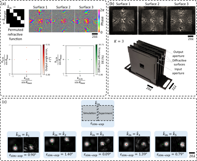
a Top: a permutation refractive function (left) and the learned phase profiles of the three diffractive surfaces used to implement this permutation refractive function (right). Bottom: numerically evaluated output angle error and diffraction efficiency for each input direction. b Fabricated diffractive surfaces (top) and the 3D-printed assembly used for experimental testing (bottom). The assembly comprises the fabricated surfaces aligned between the input and output apertures. c Comparison between simulated and experimentally measured output intensity patterns 160 mm away from the output aperture for the five different input directions. The green dot marks the center \(\left({{\mathrm{0,0}}}\right)\) of the FOV, and the red dot marks the first moment of the diffracted intensity pattern. The measured angular deviation \({\varepsilon }_{{sim}-\exp }\) remains below 1.4° in all cases, demonstrating close agreement between the simulations and experimental results.