
In this section, the simulation results are presented to evaluate the performance of the proposed DRL-based method. Various network configurations and node densities are considered to demonstrate the effectiveness and scalability of the method. The investigated Q-learning algorithm is modeled with continuous states in Python. The environment is a square space with dimensions of \(200 \times 200 \, \text {m}^2\), with a base station installed at its center (\(100 \, \text {m}, 100 \, \text {m}\)). The distribution of sensor nodes is non-uniform in each simulation, resulting in clusters with varying numbers of nodes. Each sensor node starts with \(0.5 \, \text {J}\) of energy, and the selection of each cluster head is random with a probability of 0.2. Network performance is evaluated by measuring the rate of successfully transmitted packets to the base station, which serves as the primary metric for throughput. To assess scalability and robustness, simulations are conducted for networks of different sizes, specifically with 100, 80, 60, 40, and 20 sensor nodes. It is assumed that there is no static energy consumption, which is set to 0 in the simulation, and the energy consumed by the battery itself is ignored. For simplicity, an ideal battery is assumed, and environmental noise is not modeled. Energy harvesting is based on solar input, using real irradiance data to reflect realistic energy dynamics. Throughput is measured by the number of packets successfully delivered to the base station. Communication parameters and energy model values used in the simulations are detailed in Table 1.
Table 1 System parameter settings.
According to the results, the proposed DRL-based method significantly improves throughput compared to RL-based techniques. One of the key factors contributing to the superior performance of DRL is its ability to handle continuous state spaces more effectively than Q-learning. Notably, the DRL method’s ability to adapt to fluctuating energy levels results in a more robust and efficient data flow, especially in scenarios with high sensor node variability. This analysis highlights the importance of continuous state representation in enhancing EH-WSN performance. Furthermore, the DRL-based method, by leveraging deep neural networks, can handle continuous state spaces directly. It learns to approximate the Q-values (or policies) through the neural network, enabling the agent to make decisions without needing to discretize the state space. This results in more accurate decision-making, faster convergence, and significant improvements in throughput. To check the compatibility of this algorithm with different numbers of nodes, five networks with different numbers of sensors that have random distribution in the environment have been considered. Figure 2 illustrates that the network throughput has increased in the DRL-based method compared to the RL-based method with any number of nodes. This figure displays the performance of a sensor node after 550 episodes.
Fig. 2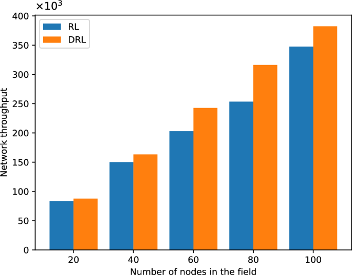
Comparison of throughput in WSN network.
Figure 3a–e illustrate the progressive improvements in packet transmission rates, highlighting the advantages of continuous energy analysis. Figure 3a shows the network throughput for 100 sensors in RL and DRL-based methods during the training process of all 100 nodes for 700 iterations. The DRL-based method increases the total number of packets sent over the network. Thus, the number of packets in 100 nodes using the RL-based method has approximately increased from 330,000 to 370,000 in the DRL-based method. This shows that sending 370,000 packets to the base station performs best for the current network configuration. These measurements can also be seen in Fig. 3b–e for nodes 80, 60, 40, and 20, respectively, which demonstrates a significant increase in each packet transmitted to the base station in the DRL-based method compared to the RL-based method. This value has approximately reached from 210,000 to 310,000 for 80 nodes, 200,000 to 242,000 for 60 nodes, 150,000 to 163,000 for 40 nodes, and from 83,000 to 87,000 for 20 nodes.
Fig. 3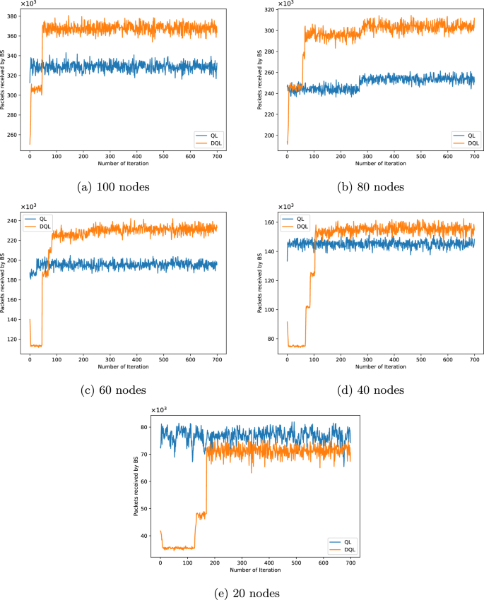
The quantity of packets that the base station has received for 100, 80, 60, 40, and 20 nodes.
As shown in Fig. 4, the packet loss results for networks with 20, 40, 60, 80, and 100 nodes are presented, respectively. Although a relative increase in packet loss is observed in the DRL-based method, the number of successfully received packets also increases. This indicates that the DRL algorithm, by optimizing decision-making and transmission scheduling, improves overall data transmission efficiency. In other words, while network traffic and, consequently, packet loss rate increase, the overall network performance in data delivery improves, leading to higher throughput.
Fig. 4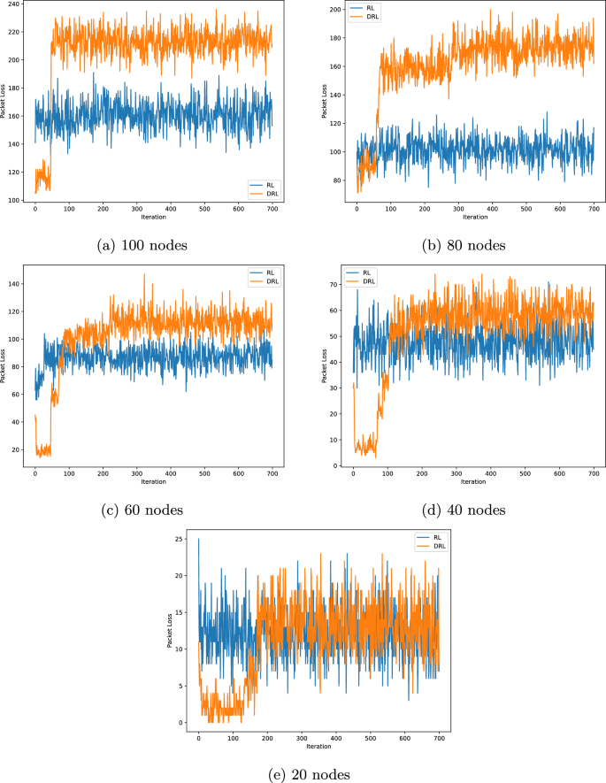
Packet loss for 100, 80, 60, 40, and 20 nodes.
Considering Fig. 3, which illustrates the number of packets received at the base station, despite the higher packet loss rate in the DRL method compared to the RL method, the network throughput is increased. This suggests that the DRL algorithm utilizes network resources more effectively, transmitting a greater number of packets. Although some packets are lost due to increased traffic or network congestion, the total number of successfully delivered packets to the destination exceeds that of the RL method. Therefore, the increased packet loss rate does not necessarily imply reduced performance but rather reflects the DRL method’s maximized exploitation of the network capacity.
Furthermore, Fig. 5a–i show the remaining energy (in Joules) of the sensor nodes in the 550th training iteration for networks of 100, 80, 60, 40, and 20 nodes, respectively. From rounds 170 to 240, the energy of the sensor is reduced because it is placed at night, during which the amount of energy that can be collected is also reduced. Figure 5b demonstrates the transmission rate (packets/round) of the sensor node in the 550th episode of rounds 1–240. Up to the 50th round, the sensors try to increase the transmission rate to the base station. However, with the decrease in energy, the transmission rate of the sensor node also decreases. As the energy levels of the sensor node progressively rise, the transmission rate also increases. The sensor node tries to set the count of packets transmitted in each round to 24. The quantity of sent packets per round is finally set to 27 for networks with 60, 40, and 20 sensors, respectively, as shown in Fig. 5d,f,h,j.
Fig. 5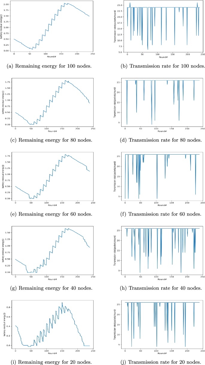
The amount of remaining energy in each round and the quantity of packets sent for different node numbers.