Experimental setup
The experimental setup is shown in Fig. 1a. A butterfly laser diode emitting at a wavelength of 1544.53 nm is sent to a pulse shaping unit that uses an amplitude electro-optic modulator (EOM) to carve two sequential rectangular pulses with a time duration of 800 ps, a delay τ = 20 ns, and a repetition rate of 20 MHz. Based on their time of emission with respect to an electronic trigger carrying the 20 MHz clock, the two pulses define the early (E) and the late (L) temporal modes. After amplification and background laser noise removal, light is coupled to the chip by using an Ultra-High Numerical Aperture (UNHA7) fiber. The optimized coupler and the use of index-matching gel reduce the coupling loss to ~1 dB/facet and ensure mechanical stability (Q ~ 8 × 10⁵ and a measured escape efficiency of ~0.75. The pump resonance is tuned to the wavelength of the input laser using a thermal phase shifter placed on the top of the resonator. The signal and idler modes used in the experiment are at a wavelength of λs,1 = 1550.9 nm (νs,1 = 193.3 THz) and λi,1 = 1538.18 nm (νi,1 = 194.9 THz). By assuming nearly single-mode spectral emission, the state \(\left\vert \Psi \right\rangle\) at the output of the chip can be written as
$$\left\vert \Psi \right\rangle =\left({e}^{{\xi }_{{E}_{1}}{a}_{{E}_{1}}^{\dagger (s)}{a}_{{E}_{1}}^{\dagger (i)}+{\xi }_{{L}_{1}}{a}_{{L}_{1}}^{\dagger (s)}{a}_{{L}_{1}}^{\dagger (i)}-{\rm{h.c.}}}\right)\left\vert {\rm{vac}}\right\rangle ,$$
(1)
where \({a}_{E/L,1}^{\dagger (s/i)}\) is the creation operator of the signal/idler photon in the early/late temporal mode at the resonance frequency νs/i,1. \({\xi }_{{E}_{1}}\) and \({\xi }_{{L}_{1}}\) are the corresponding squeezing parameters. In our case the two pump pulses have equal intensity, and their time separation is sufficiently long to reset the state of the resonator between the pulses. Therefore, one has \({\xi }_{{E}_{1}}={\xi }_{{L}_{1}}=\xi\). At the output of the chip, the pump is suppressed using a bandpass filter and the signal and idler modes are sent to an interferometer that allows one to manipulate their state. Its architecture is a fiber-based Mach–Zehnder interferometer54 in which an electro-optic phase modulator (PM) is inserted in both arms. A ~ 4m-long fiber introduces a time delay of 20 ns between the two paths, matching the time separation between the pump pulses. The unbalanced interferometer is used to mix the temporal modes, while the PMs, driven by a 18.2 GHz tone and with a modulation index of δ ~ 1.4, scramble the frequency modes. The modulation frequency corresponds to the minimum resolution of our waveshaper unit, while the choice of the modulation index allows us to equalize the scattering strength of photons to the first-order sidebands compared to that in the baseband55. The relative phase x between the long and short arm of the interferometer can be controlled, and it is stabilized using the backward-propagating pump laser as reference in an active feedback loop implemented via a FPGA board. Due to the time-energy entanglement of the photon pairs generated in the SFWM process, the locking of the pump phase stabilizes the joint relative phase of the signal and the idler photon between the long and the short path of the interferometer.
Fig. 1: Experimental setup and characterization of the squeezed light source.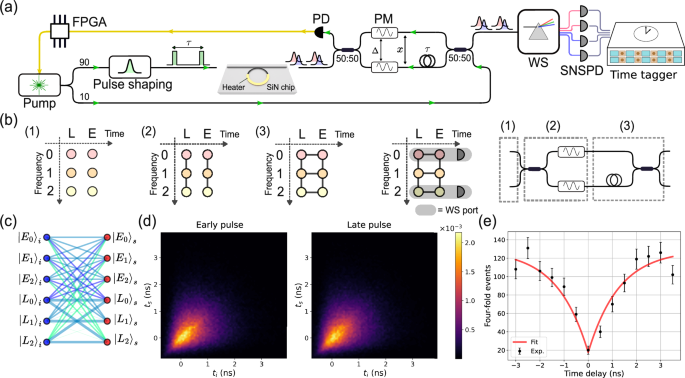
a Sketch of the experimental setup. The pump laser is shown in green, while the signal and idler modes are represented by red and blue pulses respectively. FPGA Field Programmable Gate Array, PM phase-modulator, WS waveshaper, PD photodiode, SNSPD superconducting nanowire single photon detector. b Connectivity imparted by the interferometer to the six time-frequency modes represented by a 3 by 2 rectangular lattice of points. From left to right, the initially unconnected lattice (1) develops vertical (2) and horizontal (3) edges by subsequent coupling frequency and time modes. The modes at the output of the interferometer are frequency demultiplexed to separate SNSPDs. c An illustrative example of a graph that can be encoded in the GBS experiment. The width of the edges represents the module of the complex weight, while the color encodes its phase. d Joint temporal intensity of photon pairs generated in the early and late pump pulses. e Four-fold coincidences (black) in the heralded HOM experiment as a function of the time-delay between the two heralded photons. The solid red line is a fit of the data which uses Eq. (2).
At the output of the interferometer, a programmable waveshaper is used to select the frequencies of the signal and idler photons that are detected. The detection is performed using four superconducting nanowire single-photon detectors (SNSPD) with a detection efficiency of 85%.
Characterization of the photon source
High-visibility multi-photon interference requires indistinguishable and pure photons52,56. When photon pairs are generated by SFWM in a microresonator, high spectral purity is obtained when the pump pulse has a temporal duration larger than the dwelling time of light in the cavity. From the loaded quality factor Q and the pump frequency νp, the estimated dwelling time is Q/(2πνp) ~ 660 ps. We work with a pulse duration of 800 ps, which optimizes the pulse shape carved by the amplitude EOM. The characterization of the spectral purity of the photons within each TMS is done by measuring the joint temporal intensity (JTI)51. The JTI is reconstructed by measuring the arrival times of the signal and idler photons with respect to the 20 MHz electronic trigger and by binning the timestamps into a two-dimensional grid with a resolution of 70 ps × 70 ps, which is limited by the jitter of our detectors. The JTIs of the early and late temporal modes are measured to discern any distinguishability between photons generated in the first or in the second pulse. The two JTIs are reported in Fig.1c. Their shape has been already discussed in ref. 51. The overlap between the two distributions is an upper bound to the indistinguishability, and is 0.985(2). From the JTI it is also possible to determine an upper bound to the purity \({\mathcal{P}}\) of the generated photons, which is 0.928(5) for those of the early pulse and 0.93(1) for those of the late pulse51. This value is very close to the theoretical limit achievable with a resonator source having signal, pump and idler resonances with the same quality factor, and without pump engineering57.
The purity is also estimated by performing HOM interference between photons heralded in different temporal modes. In this experiment, the idler photons at the output of the chip are sent to a 50/50 beamsplitter, while the signals are sent to the interferometer, and detected at the two output ports. The idlers herald two signal photons at the input of the interferometer with a relative delay τ. By post-selecting the events in which two signal photons exit the two output ports of the interferometer in the late time-bin, we select the cases in which they arrived at the output beamsplitter from different ports and at the same time, a scheme of the experiment is report in Supplementary Section II of the Supplemental document. To assess the visibility of the HOM dip, we varied the delay \({\tau }^{{\prime} }\) between the first and the second pulse without modifying the time delay of the interferometer. This introduces a time difference \(\Delta \tau ={\tau }^{{\prime} }-\tau\) in the arrival of the two photons at the output beamsplitter. In order to mitigate the emission of multiple pairs from each source, the pump power is regulated to achieve a pair generation probability per pulse ~0.03. The number of four-fold coincidences Nc as a function of Δτ is shown in Fig.1d. We fit the data using the model equation
$${N}_{c}=B\left(1-V{e}^{-| \Delta \tau | /{\tau }_{c}}\right),$$
(2)
where V is the visibility of the HOM dip, τc is the resonator dwelling time and B is the maximum rate of four-fold detections. The choice of Eq. (2) is motivated by the lorentzian lineshape of the signal/idler resonances (which is a decaying-exponential in the time-domain) and by the use of a rectangular pump pulse to trigger the SFWM process. The raw visibility extracted from the fit is 0.86(3). The visibility of the HOM dip is mainly limited by thermal-noise and by the spectral purity of the heralded photons (see Supplementary Section II of the Supplemental document), indicating the absence of phase correlations in the complex joint temporal amplitude38,51. We also performed the HOM interference between photons heralded from different pulses when their frequency is changed by the PMs before interfering at the output beamsplitter. The frequency of the photon in the early(late) pulse is changed by the PM placed in the long(short) of the interferometer. The two frequencies are νs/i,0 = νs/i,1 − Δν and νs/i,2 = νs/i,1 + Δν, with Δν = 18.2 GHz. We measured a HOM visibility of 0.8(1) for νs/i,0 and 0.91(5) for νs/i,2, which confirms that the two PMs do not change the Lorentzian spectra of the heralded photons when they are scattered into the same frequency-bin.
Bipartite GBS experiment
The state in Eq. (1) is sent at the input of the interferometer shown in Fig. 1a, which allows us to couple both time and frequency modes. The PMs inserted in the arms of the interferometer can scatter photons to different frequencies νs/i,j = νs/i,1 + (j − 1)Δν with an efficiency ∣Jj−1(δ)∣2, where Jj(δ) is the Bessel function of the first kind of order j evaluated at the modulation index δ. For the moderately low modulation index used in the experiment (δ ~ 1.4), most of the energy is scattered into three frequency modes, which are j = 0, 1, 2.
Events for which photons are scattered out of these frequencies are discarded. In principle, a larger modulation depth enables the coupling of more frequencies, thereby increasing the number of modes. However, we focused on only three frequency modes, as this choice limits the number of output patterns in the GBS experiment, allowing us to accumulate sufficient multi-photon events to reconstruct the output probability of each pattern. The six modes that are coupled by the interferometer can be labeled as \({\vert {E}_{j}\rangle }_{s(i)}\) and \({\vert {L}_{j}\rangle }_{s(i)}\), where E(L) labels the early (E) and late (L) temporal modes, j = (0, 1, 2) the frequency bin, and where we order the signal(idler) modes as \({\{\left\vert {E}_{0}\right\rangle ,\left\vert {E}_{1}\right\rangle ,\left\vert {E}_{2}\right\rangle ,\left\vert {L}_{0}\right\rangle ,\left\vert {L}_{1}\right\rangle ,\left\vert {L}_{2}\right\rangle \}}_{s(i)}\). To better understand the connectivity between the optical modes realized by the interferometer, one can refer to the series of transformations shown in Fig. 1b. The six time-frequency modes of either the signal or the idler photon can be arranged in a 3 by 2 rectangular grid (Fig. 1b,1). The modes in each row have different frequencies (ν0, ν1, ν2), while those in each column correspond to a different time bin (early (E) or late (L)). After the first beamsplitter, the PMs mix different frequencies within each temporal mode, thus creating vertical edges between modes in the same column (Fig. 1b,2). The subsequent fiber loop and the second beamsplitter couples the different temporal modes of the same frequency, creating horizontal edges between modes in the same row (Fig. 1b,3). This operation increase the dimensionality of the lattice by one, thereby corresponding to a non-local interaction between modes48. At the output of the interferometer, the network connectivity between time-frequency modes is represented by a two-dimensional rectangular lattice. Four-photon events, consisting of two signal and two idler photons, are post-selected in distinct frequency modes at the output of the interferometer using a waveshaper (Fig. 1a, b). The signal and idler photons then undergo separate two-photon interference patterns. Altough multi-photon interference could, in principle, be observed in six-fold events, their occurrence rate was too low to accumulate sufficient statistics due to losses in our optical components. In general, there are \((\begin{array}{c}N+k-1\\ k\end{array})\) distinct ways in which k identical photons can be arranged in N modes. For instance, considering 4 indistinguishable photons in 6 modes, one has \((\begin{array}{c}6+4-1\\ 4\end{array})=126\) possible combinations. However in our work, since signal and idler photons are distinguishable, when considering 4 photons we have for two indistinguishable signals and two indistinguishable idlers \({(\begin{array}{c}6+2-1\\ 2\end{array})}^{2}=441\) possible output patterns. Yet, not all of these patterns can be observed with our experimental setting. The use of threshold detectors implies that only collision-free events, with no more than one photon in each mode, can be distinguished. Moreover, given that the time-bin separation is smaller than the dead-time of the detectors (~80 ns), only one temporal mode can be detected for each frequency. The observable combinations have the form \({\left\vert {X}_{m}{Y}_{n}\right\rangle }_{s}{\left\vert {X}_{p}^{{\prime} }{Y}_{q}^{{\prime} }\right\rangle }_{i}\), with \(X,{X}^{{\prime} }\) and \(Y,{Y}^{{\prime} }\,\in \{E,L\}\) and m, n, p, q ∈ {0, 1, 2} with m ≠ n and p ≠ q. Out of the 441 combinations, those which satisfy these requirements are 144. While only ~30% of the total combinations can be observed with the current experimental setting, the fraction of non-collision events increases with the number of frequency modes MF, reaching the dilute sampling regime (no more than one photon in each mode) in the limit MF → ∞. Moreover, even with the current value of MF = 3, the fraction of observable combinations could be increased to ~70% by monitoring both outputs of the interferometer (see Supplementary Section V of Supplemental document). In practice, this was not possible because only four detectors were available.
To calculate the probability of observing a particular output pattern S = (Xm, Yn, Xp, Yq), we map the experiment into an instance of bipartite Gaussian boson sampling50, in which two-mode squeezers over N modes are sent at the input of an interferometer described by a 2N × 2N complex matrix Tsi = Ts⨁Ti, where Ts(i) is a N × N matrix describing the transformation of the interferometer on the signal(idler) photon. The probability of observing S is given by26
$$p(S)=\frac{{\rm{Perm}}({C}^{{\prime} }){| }^{2}}{\sqrt{\det ({\sigma }_{Q})}},$$
(3)
where \(\det ({\sigma }_{Q})={\cosh }^{4}\xi\)10 and \({C}^{{\prime} }\) can be obtained from the matrix C
$$C={T}_{i}\left(\mathop{\bigoplus }\limits_{k=1}^{m}\tanh ({\xi }_{k})\right){T}_{s}^{T}.$$
(4)
by selecting the entries at the intersections between the rows and columns of C indexed by the signal and idler modes in S. For example, if S = (E0, L1, E2, L2), the ordering of the modes introduced before implies that rows (1, 4) (signal mode numbers \(\left\vert {E}_{0}\right\rangle =1\) and \(\left\vert {L}_{1}\right\rangle =3\)) and columns (3, 6) (idler mode numbers \(\left\vert {E}_{2}\right\rangle =3\) and \(\left\vert {L}_{2}\right\rangle =6\)) are selected, which identify the following entries: \({C}_{11}^{{\prime} }={C}_{13},{C}_{12}^{{\prime} }={C}_{16},{C}_{21}^{{\prime} }={C}_{4,3},{C}_{22}^{{\prime} }={C}_{4,6}\). In writing Eq. (3) we implicitly assumed that no more than one photon is detected in each mode. It is worth to stress that Eq. (3) holds only when the modes \({S}^{{\prime} }\ne S\) are post-selected to be all in vacuum state and lossless photon number resolving detection is performed over the S modes10. However, as detailed in Supplementary Section III of the Supplemental document, for the moderate squeezing strength of the experiment, Eq. (3) provides an excellent approximation to the exact output probability. Equation (3) can be rewritten as
$$p(S)=\frac{| {\rm{Haf}}({{\mathcal{A}}}^{{\prime} }){| }^{2}}{\sqrt{det({\sigma }_{Q})}},$$
(5)
where \({\rm{Haf}}({{\mathcal{A}}}^{{\prime} })\) denotes the Hafnian of the matrix
$${{\mathcal{A}}}^{{\prime} }=\left[\begin{array}{cc}0&{C}^{{\prime} }\\ {C{}^{{\prime} }}^{T}&0\end{array}\right],$$
(6)
By using the relation between the calculation of the Hafnian and perfect matchings on graphs10, the matrix \({{\mathcal{A}}}^{{\prime} }\) can be interpreted as the complex adjacency matrix of a bipartite graph, where the two vertex sets are formed by respectively the signal and the idler modes. As it will be shown later, the graph associated with the experiment is a complete bipartite graph. An example is shown in Fig.1a for a particular setting of the PMs and interferometer phases.
The matrices Ts and Ti describing the action of the interferometer on the time-frequency modes have the general form
$${T}_{s(i)}=\frac{1}{2}\left[\begin{array}{cccccc}\cdot &{J}_{-1}^{E}&\cdot &\cdot &\cdot &\cdot \\ \cdot &{J}_{0}^{E}&\cdot &\cdot &\cdot &\cdot \\ \cdot &{J}_{1}^{E}&\cdot &\cdot &\cdot &\cdot \\ \cdot &{J}_{-1}^{L}&\cdot &\cdot &{J}_{-1}^{E}{e}^{i{\theta }_{1}^{s(i)}}&\cdot \\ \cdot &{J}_{0}^{L}&\cdot &\cdot &{J}_{0}^{E}{e}^{i{\theta }_{2}^{s(i)}}&\cdot \\ \cdot &{J}_{1}^{L}&\cdot &\cdot &{J}_{1}^{E}{e}^{i{\theta }_{3}^{s(i)}}&\cdot \end{array}\right],$$
(7)
where \({J}_{i}^{E(L)}\) is the Bessel function of the first kind of order i describing the strength of the electro-optic modulation of the PM inserted in the short (E) and long (L) arm of the interferometer. The matrix entries denoted with dots are not relevant for calculating the outcome probabilities because photons enter into the interferometer only at frequencies νs/i,1. The factor 1/2 in Eq. (7) accounts for the two 50/50 beamsplitters forming the interferometer. According to ref. 58, two matrices M and \({M}^{{\prime} }\) describe the same physical interferometer if they are related by \(M={D}_{1}{M}^{{\prime} }{D}_{2}\), where D1 and D2 are diagonal matrices describing pure phase shifts on the modes. This feature allows one to consider real entries in a particular row and column, corresponding to a reference mode. We chose the second mode as reference, ans take all the entries of the second column as real numbers. The phases \({\theta }_{j}^{s(i)}\) are the phase differences between the short and long path of the interferometer for the signal(idler) photon whose frequency has been changed by the PM from νs/i,1 (before entering the interferometer) to νs/i,j (after leaving the interferometer). These phases also embed the relative phase between the two TMS.
While Ji can be determined by injecting a laser at the input of the two PM and by measuring the intensity of the ith sideband at the output, the phases \({\theta }_{j}^{s(i)}\) require further considerations. In particular, since the interferometer is locked to a fixed value of the phase of the pump θp and not to an absolute reference, \({\theta }_{1}^{s(i)}\) fluctuates over time but \({\theta }_{1}^{s}+{\theta }_{1}^{i}=2{\theta }_{p}\) is given by the phase matching condition of spontaneous FWM54. The phases associated to the signal and idler photons that have changed their input frequencies from νs(i),1 to νs,j = νs,1 + (j − 1)Δν and νi,k = νi,1 + (k − 1)Δν after the PMs satisfy \({\theta }_{j}^{s}+{\theta }_{k}^{i}=2{\theta }_{p}+2\left(\frac{j+k}{2}-1\right)\Delta\), where Δ is a phase which depends on Δν and on the relative phase between the two RF signals driving the two PMs. Following these arguments, we can insert Eq.(7) into Eq.(4) and write the matrix C as
$$C=\frac{{\bar{J}}^{2}}{4}\left[\begin{array}{cc}{{\mathbb{1}}}_{3}&{{\mathbb{1}}}_{3}\\ {{\mathbb{1}}}_{3}&{C}_{LL}\end{array}\right],$$
(8)
where \({{\mathbb{1}}}_{3}\) is a 3 × 3 matrix filled by ones and the block CLL is given by
$${C}_{LL}=\left[\begin{array}{ccc}1+{e}^{i(x-2\Delta )}&1+{e}^{i(x-\Delta )}&1+{e}^{ix}\\ 1+{e}^{i(x-\Delta )}&1+{e}^{ix}&1+{e}^{i(x+\Delta )}\\ 1+{e}^{ix}&1+{e}^{i(x+\Delta )}&1+{e}^{i(x+2\Delta )}\end{array}\right],$$
(9)
where \(x=2{\theta }_{p}+\arg ({\xi }_{{L}_{1}}/{\xi }_{{E}_{1}})\) and we have set \({J}_{i}^{E/S}=\bar{J}\) for i = (0, 1, 2). This condition is achieved by the particular choice of the modulation index δ = 1.4 in the experiment. Hence, from Eq. (3) and Eqs. (8) and (9) one has that the probability of detecting a signal-idler pair in the modes q and p, respectively, is given by ∣Cqp∣2. From Eqs. (8) and (9) one can also see that the output of the interferometer only depends on the parameters x and Δ. The parameter x can be controlled by changing the pump phase θp at which the interferometer is locked. The parameter Δ depends on the phase offset between the RF signals driving the PMs, and can be determined by measuring two-fold coincidences between the signal and idler photons at frequencies [j, k] = [νs,1 + (j − 1)Δν, νi,1 + (k − 1)Δν] and detected in the late time-bin.
From Eqs. (3) and (9) the coincidence probability pjk is given by
$${p}_{jk}\propto 1+\cos \left(x+2\left(\frac{j+k}{2}-1\right)\Delta \right).$$
(10)
Scanning x yields an interference fringe with an offset that is a multiple of Δ. There are \((\begin{array}{c}4\\ 2\end{array})=6\) possible combinations of signal and idler frequencies, which are ([0, 0], [0, 1], [0, 2], [1, 1], [1, 2], [2, 2]), with respective offsets (− 2Δ, − Δ, 0, Δ, 2Δ). Note that the value of Δ can be modified by changing the relative phase of the RF signals driving the two PMs. Equation (10) can be interpreted as a generalization of the more familiar Franson-type interference, in which photons are allowed to change their frequency. The interference is associated with the photon pairs that are generated in the early pump pulse and travel the long path of the interferometer, and those generated in the late pulse that travel the short path. Even if the PMs change the frequency of the signal or idler photon, these events are still indistinguishable and their amplitude probabilities interfere. In Fig. 2 we report an example of measurement of the interference fringes for all the six combinations of signal-idler frequencies. All curves are fit using Eq. (10), leaving Δ as a free parameter. As expected, there is no offset between the curves relative to the frequency combinations [1, 1] and [0, 2]. On the contrary, the combinations [0, 0] and [0, 1] have offsets − 2Δ and − Δ, while the combinations [1, 2] and [2, 2] have offsets Δ and 2Δ.
Fig. 2: Characterization of the time-frequency interferometer.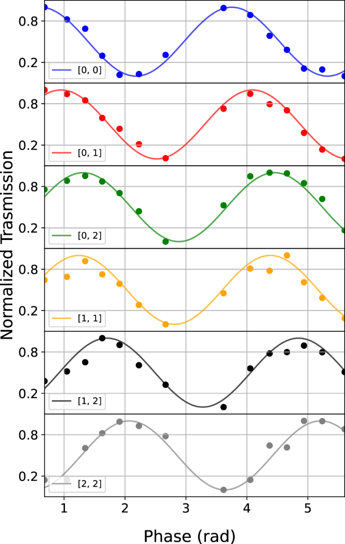
Coincidence probabilities pjk between the signal and the idler photons at frequencies [j, k] = [νs,1 + (j − 1)Δν, νi,1 + (k − 1)Δν] detected in the late time-bin as a function of the interferometer phase. The datasets have been normalized for clarity. Solid lines are fit of the data which use Eq.(10).
After the characterization of the interferometer, we sampled the 144 four-photon patterns at the output for four different values of x and Δ, and compared the number of collected events to those predicted by Eq. (3). The experiments are performed by setting the average number of photons per pulse to ~ 0.1, corresponding to a squeezing parameter of ∣ξ∣ ~ 0.3. The total integration time for each setting (x, Δ) is 13 hours.
The measured and predicted output patterns are shown in Fig. 3a and are in very good agreement. The fidelity \({\mathcal{F}}\) between the theoretical and experimental probability distributions pth and \({{\boldsymbol{p}}}^{\exp }\), defined as
$${\mathcal{F}}=\mathop{\sum }\limits_{i}\sqrt{{p}_{i}^{({\rm{th}})}{p}_{i}^{(\exp )}},$$
(11)
is 0.989(2) for (x = 1, Δ = π), 0.992(1) for (x = 1, Δ = 0) and 0.987(2) for (x = 1.8, Δ = − 0.16). Furthermore, we used a Bayesian approach to evaluate the posterior probability that the collected dataset is generated by alternative models than squeezed light at the input of the interferometer23. We consider three possible alternative models of input state, which are thermal states, coherent states and distinguishable TMS. We also compare the output statistics to that predicted by uniform sampling. Details on the model validation procedure can be found in Supplementary Section IV of the Supplemental document. The posterior probabilities are shown in Fig. 3b as a function of the number of samples in the dataset. For each pair of (x, Δ), the probability that the measured samples arise from any of the alternative models vanish after ~ 103 samples. This shows that the output samples are actually generated by squeezed light at the input of the interferometer.
Fig. 3: GBS output pattern probabilities and Bayesian validation of the model describing the statistic of the output samples.
a Comparison between the experimental and the theoretical predicted number of four-photon events for 144 different output patterns. The three stacked panels differ by the value of the phases (x, Δ). b Posterior probability that the collected dataset is generated by alternative models than squeezed light at the input of the interferometer as a function of the number of samples in the dataset.
Evaluation of graph similarity
It is known that a graph can be encoded in a GBS experiment through a correspondence between the graph’s adjacency matrix and the combination of an interferometer with squeezed light16,17,53. The graphs that can be encoded in our experiment are bipartite and represented by the adjacency matrix \({{\mathcal{A}}}^{{\prime} }\) in Eq.(6), where the two vertex sets Vs = (1, . . . , 6) and Vi = (1, . . . , 6) are the signal and the idler time-frequency modes. The complex weight of an edge from a signal vertex j to an idler vertex k is given by the entry Cjk of the matrix C in Eq. (4). Given two GBS experiments encoding isomorphic graphs, any output pattern n has the same probability to occur as a pattern \({{\boldsymbol{n}}}^{{\prime} }\) that is related to n by a permutation of the modes16. Hence, one can find our if two graphs are isomorphic by comparing the output probabilities of the two experiments. The problem of determining if two graphs are isomorphic falls in the NP complexity class, which motivates the use of GBS for providing a computational speed-up over classical algorithms16. The problem of estimating a number of output probabilities that grows combinatorially with the number of vertices has been tackled in refs. 16,26, where the concepts of orbits and feature vectors on graphs are implemented. An orbit is defined as a set of output patterns that are equivalent under permutation. For example, the orbits [1, 1, 1, 1] and [1, 1] contain all the detection events where 4 photons and 2 photons are respectively detected in separate modes, without distinguishing the mode number, and with zero photons in all the other modes. Two GBS experiments encoding isomorphic graphs have identical probabilities of generating samples from the same orbit, which suggest that orbits can be combined into feature vectors whose distance depends on the degree of similarity between two graphs.
In our implementation, we set x = 1 and Δ = 0 and collected the output samples with 2 and 4 photons. From the complete bipartite graph with 12 vertices, we extracted 7 different families of graphs with 4 vertices \({\{{G}_{4}\}}_{i = 1,…,7}\), and 13 different families with 6 vertices \({\{{G}_{6}\}}_{i = 1,…,13}\), which are shown in Fig. 4c, d. Each family is formed by isomorphic graphs, but graphs belonging to different families are not isomorphic. We clustered the recorded events into two and four-photon orbits O2 and O4. More specifically, these orbits are formed by two and four-photon events while tracing out the unobserved modes, which are therefore not post-selected to contain zero photons. However, we will still refer to O2 and O4 as orbits that can be used to construct feature vectors for the purpose of graph clustering and classification. We assign to each graph its feature vector f = (N(O2), N(O4)), where N(Oi) is the number of samples in the orbit Oi, and plot the feature vectors in Fig. 4a. We see that the isomorphic graphs within each family have very similar feature vectors, thereby forming clusters. We can recognize 5 separate clusters of graphs in Fig. 4a, and 10 in Fig. 4b, corresponding to different families of non-isomorphic graphs. Therefore, the approximate orbits can be used to identify isomorphic graphs in our small scale problem. The overlapped groups (e.g., \({\{{G}_{4}\}}_{2}\) and \({\{{G}_{4}\}}_{3}\) for 4 vertex graphs and \({\{{G}_{6}\}}_{2}\) and \({\{{G}_{6}\}}_{3}\) for six vertex graphs) could be separated in principle by adding more and/or different orbits to the feature vector.
Fig. 4: Evaluation of graph similarity using two and four-photon orbits.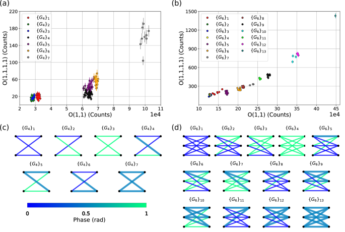
a Feature vectors corresponding to 7 different families of graphs with four vertices. The components of the vectors are the number of samples of the two and the four photons orbits O2 and O4. b Same as in (a), but relative to 13 different families of graphs with six vertices. c Representation of the 7 different families of graphs with 4 vertices. The width of the edges represents the module of the complex weight, while the color encodes its phase. d Same as in (c), but relative to the 13 families of 6 vertex graphs.